Calculus Without Tears

MATLAB, FREEMAT and OCTAVE

MATLAB is the programming language of choice for many analytical engineering projects, and all the graphs in CWT were created using MATLAB. It is also a super calculator, and all the calculations for the exercises were also done with my most convenient calculator, MATLAB. So, why have I waited till now to tell you about this fantastic tool? Because MATLAB is expensive. However, now there are free clones of MATLAB available, my favorites are FREEMAT and OCTAVE. FREEMAT and OCTAVE are totally legal and free, and can be downloaded from the web. FREEMAT and OCTAVE have all the features of MATLAB.

Click here for the FREEMAT Home Page.

Click here for the OCTAVE Home Page.

MATLAB as a Calculator

So I recommend that you download either FREEMAT or OCTAVE right now, and at a mimimum, learn to use it as a calculator. How difficult is that? When you run the program it comes up in a window and prints a prompt '>'. After the prompt, type in an expression followed by (Enter) and FREEMAT/OCTAVE will evaluate the expression and print the answer. E.g.
>10+15+81/9
34

MATLAB is much more convenient than a handheld calculator, because, if you type in a long expression and evaluate it, and then discover you've made a mistake, or you want to change it for any reason, you can enter an 'up arrow' and the previous line you entered will reappear after the prompt, and you can edit the line and reenter it. That is, you can edit only the parts you want, you don't have to retype the entire line. This makes a big difference, believe me.

MATLAB Variables and Vectors

MATLAB also has memory. A named memory location is called a 'variable'. A value is assigned to a variable ( 'a' in the line below) with an assignment command of the form
>a = 10 + 15;
A variable can also store a list of values (called a vector). The command
>b=[2.1 8 5.3 100 -10];
stores a five element list in b, the first element is 2.1, the second 8, and so on. Individual elements in a list are referenced by following the variable name with an index into the list in parentheses, thus b(1) references the first element, b(2) the second, and so on.
Typing the name of the variable after a prompt causes its value to be printed, thus
>a
25
>b
[2.1 8 5.3 100 -10]
>b(3)
5.3
b(4) = 25;
b
[2.1 8 5.3 25 -10]

MATLAB is a Programming Language

Using MATLAB as a calculator is just the beginning. It is also a programming language that is very easy to use. And I mean VERY easy. There is now (2006 onward) an appendix in each CWT volume giving a very brief introduction to MATLAB programming. One of the beauties of the language is that it was designed for scientists and engineers, and not computer programmers, so it is very 'user' oriented. Also, it has features that make it very easy to produce graphs. And, if the truth be known, drawing graphs is one of the big thrills in physics and engineering. Graphing is 'built-in' in MATLAB and only requires one line, of the form 'plot(x,y)' where x is a vector of the the horizontal coordinates of the points to be graphed and y is a vector of the vertical coordinates of the points to be plotted.

A 'for loop' causes the list of commands between the for and end commands to be executed repeatedly. The for command specifies an index variable and a list of values for the variable, the commands in the loop are executed once for each value in the index list. Example:
j=0;
for i= [1 2 3 4 5]
    a(i)=j;
    j=j+i;
end
a
[0 1 3 6 10]
Note that 'execution' of a for loop doesn't start until the end command is entered. So, when the 'end' command is entered above, the computer executes the following commands:
i=1; a(i)=j; j=j+1;    i=2; a(i)=j; j=j+i;    i=3; a(i)=j; j=j+i;    i=4; a(i)=j; j=j+i;    i=5; a(i)=j; j=j+i;

The MATLAB commands that generated the graph are shown in green below, following each command is a comment preceded by %. i and t are variables, x and y are vectors each with 1000 elements.



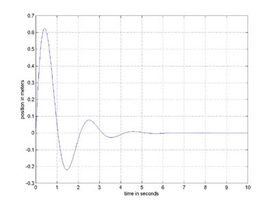
    for i=1:1000    % i is assigned values 1, 2, 3 ... 1000 in a 'for loop'
        t=i/100;    % the ith x coordinate is calculated
        x(i) = t;    % the ith x coordinate is saved
        y(i) = exp(-t)*sin(3*t);    % the ith y value is computed and saved
    end    % this ends the 'for loop'
    plot(x,y)    % draw the graph
    grid    % draw the grid on the graph
    xlabel('time in seconds')    % label the x axis
    ylabel('position in meters')    % label the y axis