
Calculus Without Tears
Synopsis of Mathematical Modeling and Computational Calculus II
The Finite Difference Method
1. Introduction
The Basic Paradigm of Mathematical Physics and Engineering
Since the time of Newton the basic paradigm of mathematical physics and engineering has been the following:
1. Understand the physical laws governing the phenomena being studied.
2. Develop a differential equation model of the process.
3. Solve the differential equations. Ay, there's the rub.
4. Analyze the results
The Need for Computational Calculus
The problem has always been step 3, as most differential equations do not have analytic solutions.
Thus, the student takes a year of calculus in high school, and then a series of courses in college consisting of differential calculus, integral calculus, multi-variable calculus, vector calculus, and culminating in a course in differential equations. So far no physical systems have been analyzed, and the student is never told that most problems can't be solved using analytic calculus. The student proceeds to a course in Fourier analysis and the Laplace transform, followed by a course in linear systems analysis, and finally, a few weeks before graduation, real systems, linear ones that is, can be analyzed analytically.
If a student takes an upper division or graduate course in dynamics, or astrorphysics, or material science, or electronics, or Maxwell's equations, or fluid dynamics, non-linear systems will be encountered, and he/she will be introduced to computational calculus, which is how most physics and engineering problems are solved today. See, for example, the online course Dynamics of Physical Systems, https://www.youtube.com/playlist?list=PLD074EEC1EBEFAEA5 , where computational calculus is introduced when it's time to solve problems, in lecture 20.
But, here is the thing, computational calculus is trivially easy and can be taught in high school. It doesn't require years of study, Euler's method, used in MMCC I, and its extension to partial differential equations, the finite difference method used in MMCC II, can be fully explained in an hour ! Then, its just a matter of practice, which is what we do in the MMCC books.
The Finite Difference Method
The finite difference method (FDM), applied to ordinary differential equations, is Euler's method, the method used in MMCC I. Given a differential equation
Euler's method substitutes an algebraic expression, essentially the expression defining the derivative, for the derivative in the differential equation, the substitution is
This is just our old favorite, velocity, df/dt, = distance f(x+dt) - f(x), divided by time, dt.
The resulting algebraic equation is then used to compute, using arithmetic operations only, solutions to the original ordinary differential equation.
The FDM applied to a partial differential equation uses the following substitutions for the partial spatial derivatives in the differential equation
And, the resulting algebraic equation is then used to compute, using arithmetic operations only, solutions to the original partial differential equation.
The salient properties of the FDM are that it is easy to learn, intuitively clear, works the same for every problem, and it is very powerful and can be used to solve a wide variety of problems.
The Program's the Thing
We follow the basic paradigm for each project in the book, starting with the physical laws, and giving a derivation of the differential equation model in baby steps, striving for intuitive clarity and transparency. At that point the FDM substitutions are made in the model, and a MATLAB/OCTAVE/FREEMAT program is written to implement the computations. So, finally, exerything in the model is made explicit, in terms of additions, subtractions, multiplications, and divisions. Writing a program enables the student to see exactly how each component of the model affects other components and how it contributes to the total solution. In addition, by varying model and system parameters, the process can be studied for a variety of model characteristics, initial conditions and disturbance functions. The program gives the student a sense of complete mastery of the mathematical analysis of the physical process.
MATLAB has excellent built-in graphing features, and the graphs below, with one exception, did not require any programming at all beyond computing the data to be graphed.
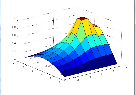
2. Heat Transfer
Physical Laws
The physical law governing heat transfer is Fourier's Heat Transfer Law, which is
Differential Equation Model of Heat Transfer
The differential equation model is derived from Fourier's Heat Transfer Law, for heat transfer in 2-D the model is
Notes: Derivation
Projects
Now we make the FDM substitutions into the model, and compute.
Notes: Computation
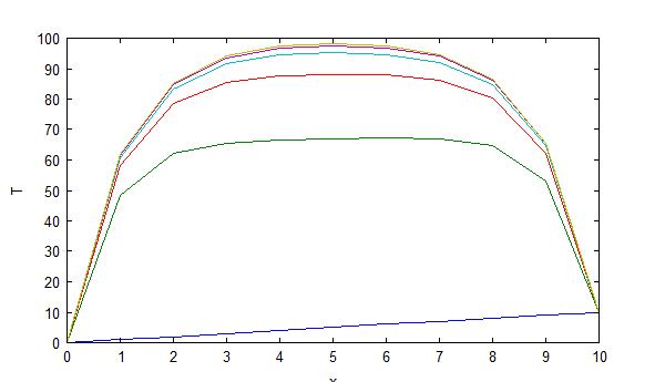
1-D heat transfer
 ...
...
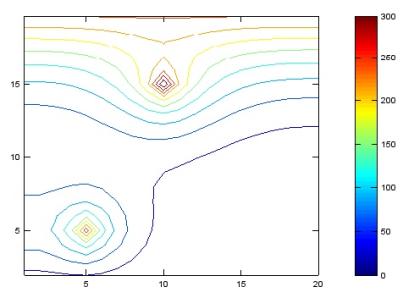
2-D heat transfer
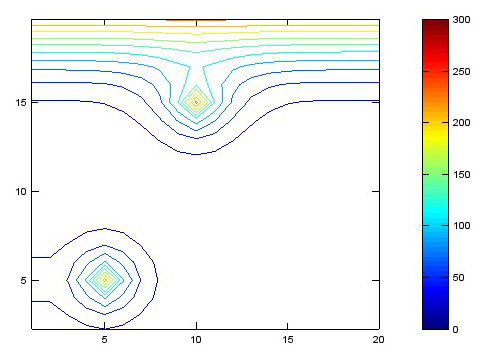 ...
...
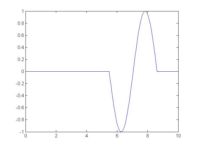
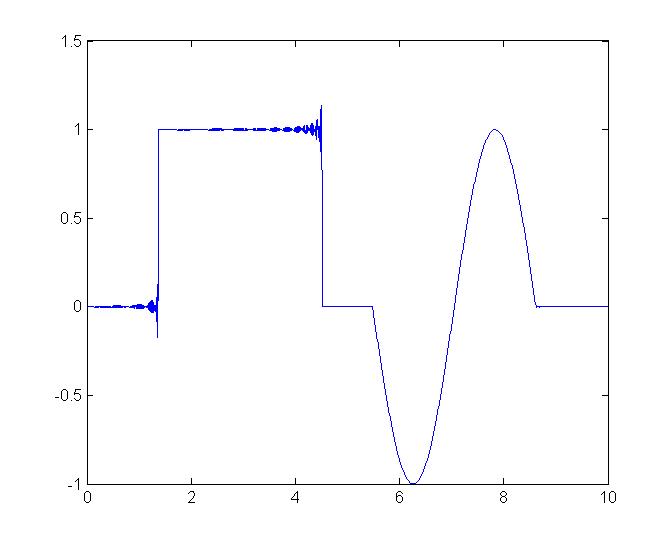
3. The Wave Equation
Physical Laws
The wave equation can be derived from a number of different physical laws, in this chapter it is derived from Newton's 2nd Law of Motion, F = MA. It is also derived from Maxwell's equations in the chapter on Maxwell's equations.
Differential Equation Model of the Wave Equation
The differential equation model for the wave equation in 2-D is
Projects
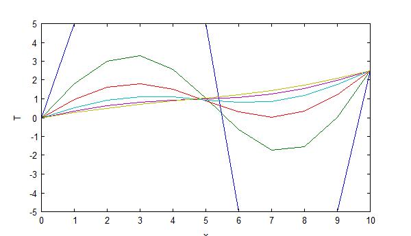
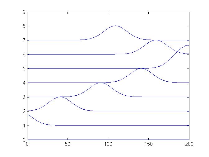
1-D wave equation
 ...
...
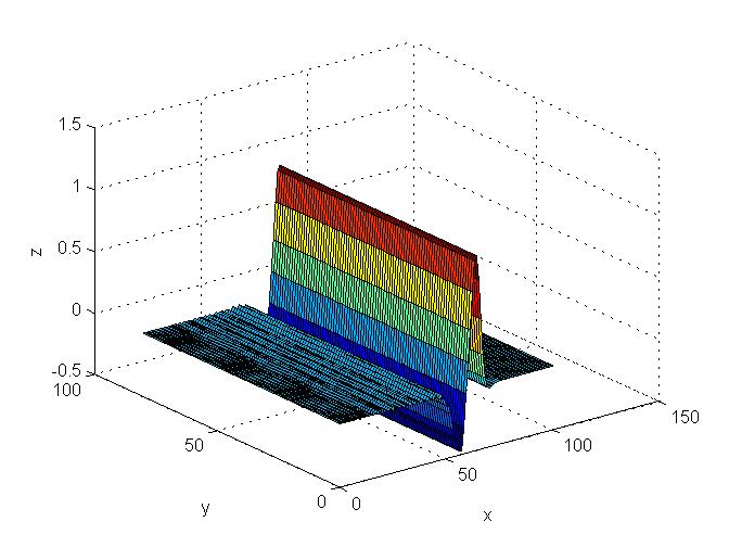
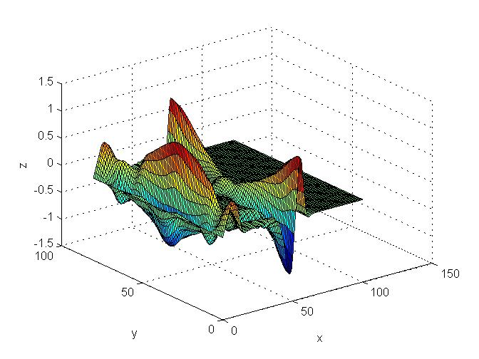
2-D wave equation
 ...
...
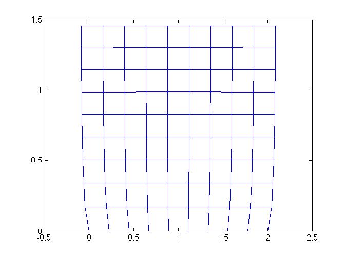
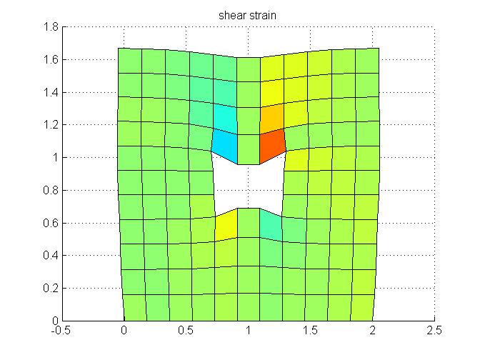
4. Stress and Strain
Physical Laws
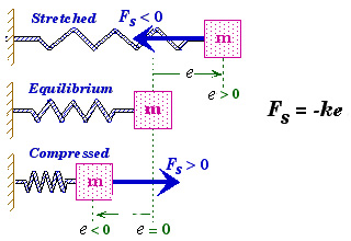
The stress and strain model is derived from Newton's 2nd Law of Motion, and Hoooke's Law. Hooke's Law in 1-D is
the familiar spring law
Things get a little more interesting in 2-D and 3-D, where there are shear strains and stresses. Hooke's Law in 2-D takes the form
where E = Young’s modulus
V = Poisson’s ratio
G = shear modulus
εx, εy, σx, σy denoting normal strains and stresses
θ, τ denoting shear strain and stress.
Differential Equation Model for Stress and Strain
The equilibrium model for stress is
Making the substitutions from Hooke's 2-D law gives the model in terms of displacements
Notes: Stress and strain tensors
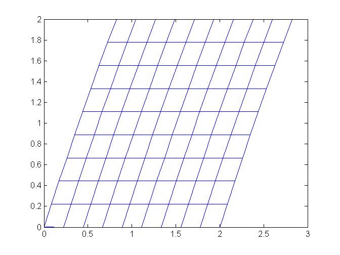
Projects
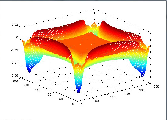
Downward force on a plate ............................................................. shear force on a plate
 ...
...
...downward force on a plate with a cutout
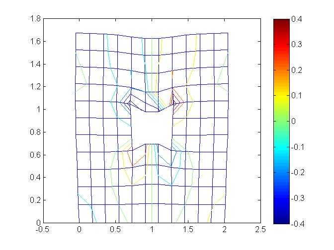 ...
...
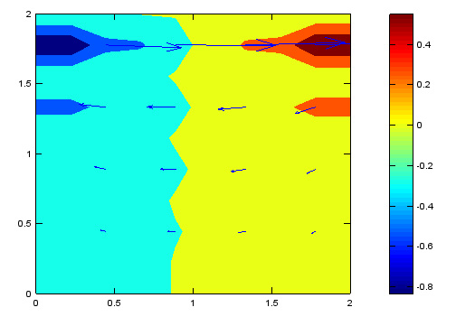
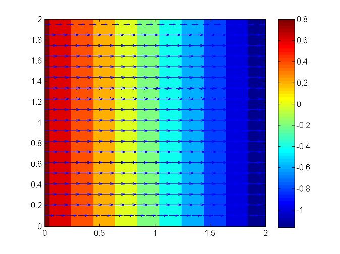
5. Fluid Dynamics
Physical Laws
The differential equation model for fluid motion, the Navier-Stokes equations, is derived from Newton's 2nd Law of Motion, the Reynold's Transport Theorem, that let's us apply Newton's 2nd law of motion to a control volume of fluid, and Newton's Law of Viscosity, that states that the shear stress is proportional to shear strain rate for fluids.
Differential Equation Model for Fluid Motion
The derivation of the Navier-Stokes equations from the physical laws is given in complete detail, the Navier-Stokes equations are
Notes: Deriving the momentum equations
Projects
Cavity flow ..................................................................................... channel flow
 ...
...
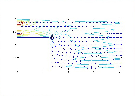
Flow over backward step
6. Maxwell's Equations and Electromagnetic Radiation
Physical Laws
Maxwell's equations in integral form follow directly from four simple experiments, descibed in detail in the book. Converting the integral equations to differential equations is straightforward. Maxwell's equations in differential form are the model equations for electromagnetic radiation, and the FDM can be used out of the box to compute solutions. The popular Yee algorithm is a modification of the FDM.
Notes: Derivation
Differential Equation Model for Electromagnetic Radiation
Maxwell's 3rd and 4th equations in differential form are the model for electromagnetic radation, in 2-D they are in expanded form
Projects
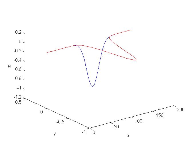
1-D electromagnetic radiation - E and B fields
 ...
...
2-D electromagnetic radiation ... a plane wave ...................... a plane wave hitting a centered metal plate
 ...
...
.... a plane wave hitting a metal plate with one hole ................. with two holes
 ...
...
7. Consistency, Stability, and Convergence
Von Neumann's Method for Stability Analysis
Examples