
Calculus Without Tears
CWT Volume 4 - Good Vibrations, Fourier Analysis and the Laplace Transform
The Fourier Philharmonic
The 1812 Overture by Tchaikovsky lasts for 14 minutes and 40 seconds. It is scored for a philharmonic orchestra having up to eighty musicians, playing a wide variety of instruments. The instruments include strings: violins, cellos, basses, brass: trumpets, trombones, French horns, tubas, woodwinds: clarinets, saxophones, flutes, piccolos, as well as percussion: drums, cymbals, bells, and triangles. The music for each instrument consists of multiple pages, each containing hundreds of notes. Each instrument gets a full workout in the course of the overture, which contains loud bombastic sections, as well as tranquil interludes.
When Joseph Fourier decided to form an orchestra to play the Overture, he had only flute players (fortuitous, as the flute plays what is close to a pure sine wave) at his disposal. And, the players were severly limited, each player could play only one note, at one volume, for the duration of the piece. So that, when Fourier's baton dropped on the initial downbeat, each player played his/her one note, and held it at a constant volume, for 14 minutes and 40 seconds, through the climatic finale.
Fourier claimed that he could re-score the piece (see how in the last section) so that his orchestra's version of the 1812 Overture would sound exactly like the full orchestra version, as played by the Berlin philharmonic, for example.
Let me suggest that you carefully re-read the previous two paragraphs a few times, to realize how absolutely unbelievable the theorem demonstrated below really is. Each player plays one note, at one volume, for the duration of the piece. Not a misprint.
Think of it this way: right before the final climatic chord, there is a second of silence. During this silence every player is playing the same note he/she has played since the beginning of the piece, at the same volume, and yet the listener hears silence; each player continues playing his/her note at the same volume through the finale, and the listener hears crashing symbols, blaring horns, strumming basses, etc. Clearly, this is not possible. Yet, it is, as we will see shortly.
Famous mathematicians of the day, (and among the greatest of all time), including Poisson, Laplace and Lagrange, thought Fourier was wrong, and told him so.
But Fourier was right. He couldn't prove it though, and the controversy raged for twenty years until Johann Dirichlet proved that Fourier's orchestra could play the 1812 Overture, and any other piece of music, and sound just like the Berlin philhamonic.
Fourier's technique of decomposing any signal into its sine wave components has become the foundation of linear analysis and engineering math, with applications in all branches of science.
Fourier Series
Here's how Fourier assembled his orchestra. Let f(t), 0<= t <= T = 2π (time normalized for convenience - the big theorem is coming and we want the notation to be as simple as possible), be the waveform of the 1812 Overture. The order n Fourier series approximation to f is given by
Sn(x)=A0+A1cos(x) +
B1sin(x) +.....+ Ancos(nx) +
Bnsin(nx)
where
A0 = 
Aj =  for j = 1,2...
and
Bj =  for j = 1,2...
Each pair of sin and cos terms above represents a note played by one of Fourier's flute players, with j cycles per the length of the piece the frequency of the note, and Aj the in-phase amplitude of the note and Bj the out-of-phase amplitude of the note.
Fourier claimed that as n increases, the series above approximates f to any desired degree of accuracy. Dirichlet proved he was right. Using only simple trig identities (covered in CWT Vol. 3), Dirichlet showed that Sn could be rewritten as
Sn(x) =
Define Dn(y)=(1/π)(1/2 + cos(y) + .... +cos(ny)) and the same trig identities can be used to show
Dn(y)= sin(ny+y/2) / sin(y/2).
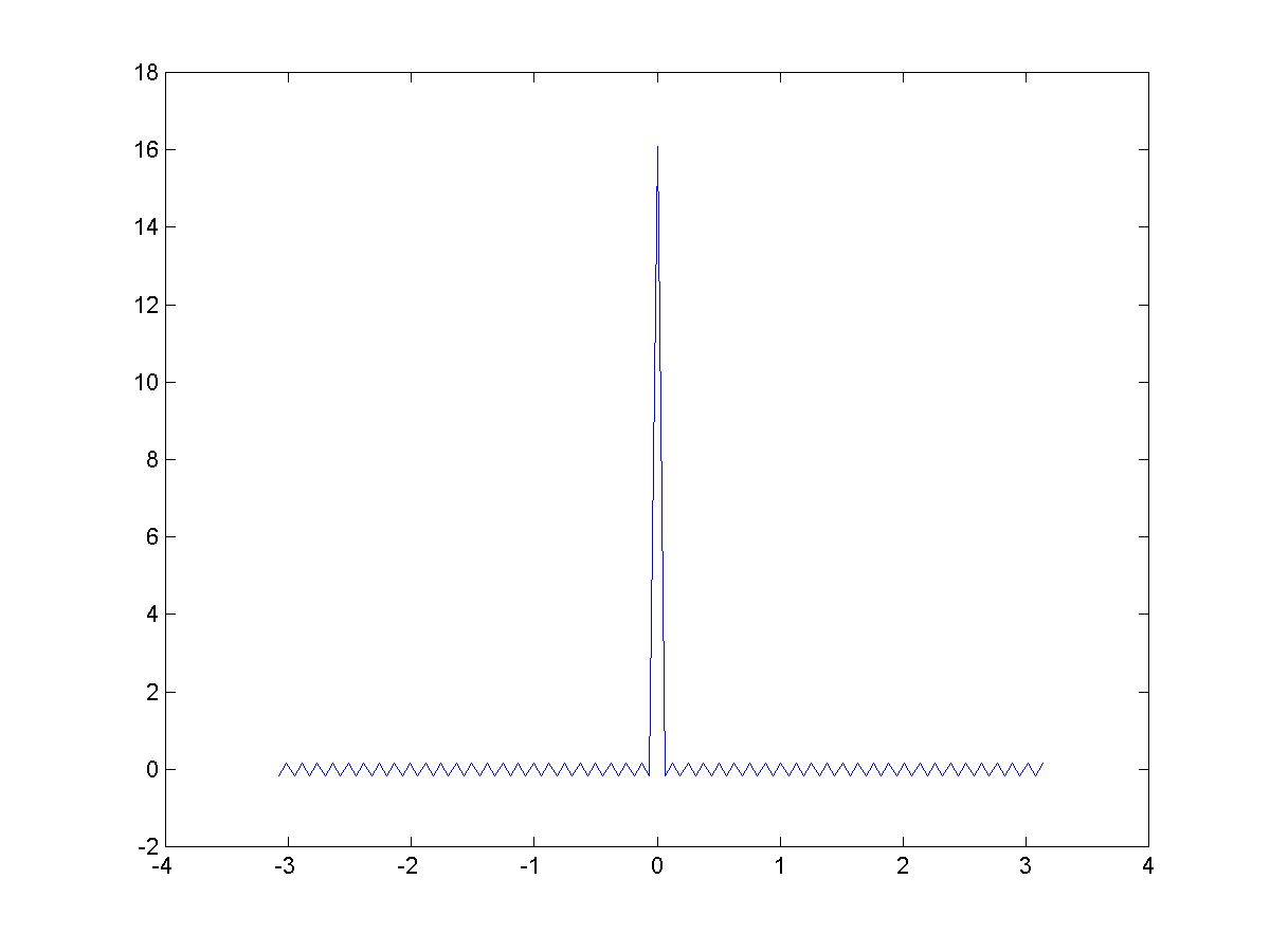
Dn for n = 50 is shown to the left.
Integrating the formula defining Dn(y) gives
and from the picture almost all the area of the integral is the central spike. As n increases Dn approaches a 0-width pulse at 0, with integral 1, so it follows that in the limit
Sn(x) = 
And, we're done ? ?? Yes, amazingly enough, we're done.
Examples of Fourier Series
 Series approximation to pulse train | 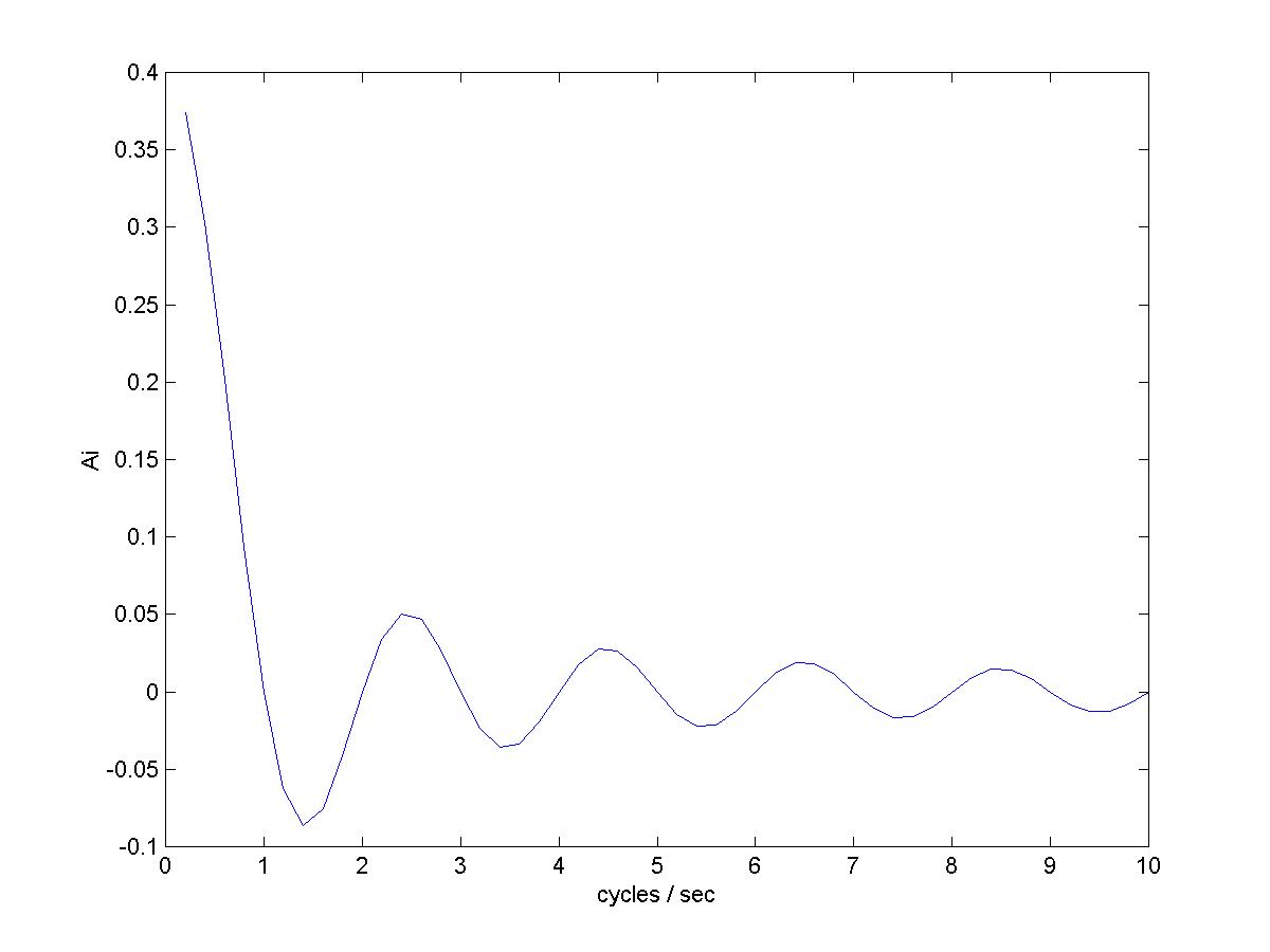 The Fourier coefficients |
Sawtooth waveform
Sines and cosines
One half cosine with period 0.5/T
Discontinuities and the Gibbs Phenomenon
The Fourier Transform and the Fourier Integral Theorem
Periodic functions can be approximated by Fourier series. This result can be extended to represent any function as an integral of sine and cosine components. Let f be a function and define fT to be the periodic extension of f on the interval -T/2 to T/2, that is, fT = f on the interval -T/2 to T/2 and fT is periodic with period T. Then fT can be approximated by a Fourier series. The Fourier series approximation uses the frequencies that are multiples of the base frequency 1/T cycles per second. As T increases, fT approaches f, and the spacing between the frequencies in the series approximations, that is 1/T, decreases. In the limit, we will need to replace the summation of the series by an integral. The integral equals f, this is the Fourier Integral Theorem. The coefficients of the sine and cosine components are given by the Fourier transform.
The Fourier transform consists of the Fourier cosine transform and the Fourier sine transform. The Fourier cosine transform of f is defined for any real frequency λ cycles/second by
Af(λ) = 
and the Fourier sine transform of f is defined by
Bf(λ) = 
The Fourier Integral Theorem (FIT) states
f(x) = 
We simplify by assuming that f(x) = 0 for x < -T0/2 and x > T0/2. We'll also assume f is even so that the sine transform is 0. The Fourier series coefficients for fT (were fT matches f for -T/2 < t < T/2, and is extended to be periodic with period T) are then
Aj = A(j/T) =  = Af(j/T)/T for j = 0,1,2...
We can approximate the FIT integral by dividing the range of frequencies into intervals of size h=1/T and summing with
 <-
<-  = Sn(fT,x)
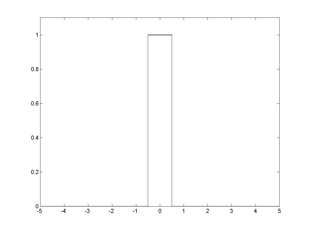
A picture shows what's happening, let f be a unit pulse centered at 0, then according to the FIT,
f(1) = 
and the graph of the integrand below shows the approximation Sn(f2,1) as shaded.
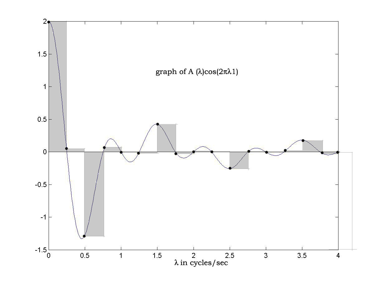 Of course the graph extends to infinity. Each shaded rectangle corresponds to a term in Sn(f2,1), and the total value of the shaded area is the limit of Sn(f2,1) as n increases which is f(1) as the Fourier series approximation to fT converges to fT(1) = f(1). As T increases the interval size decreases and the approximations approach the value of the integral, and the value of each approximation is f(1) !, hence the value of the integral is f(1) and the FIT is demonstrated.
Examples of Fourier Transforms
 A Single Pulse | 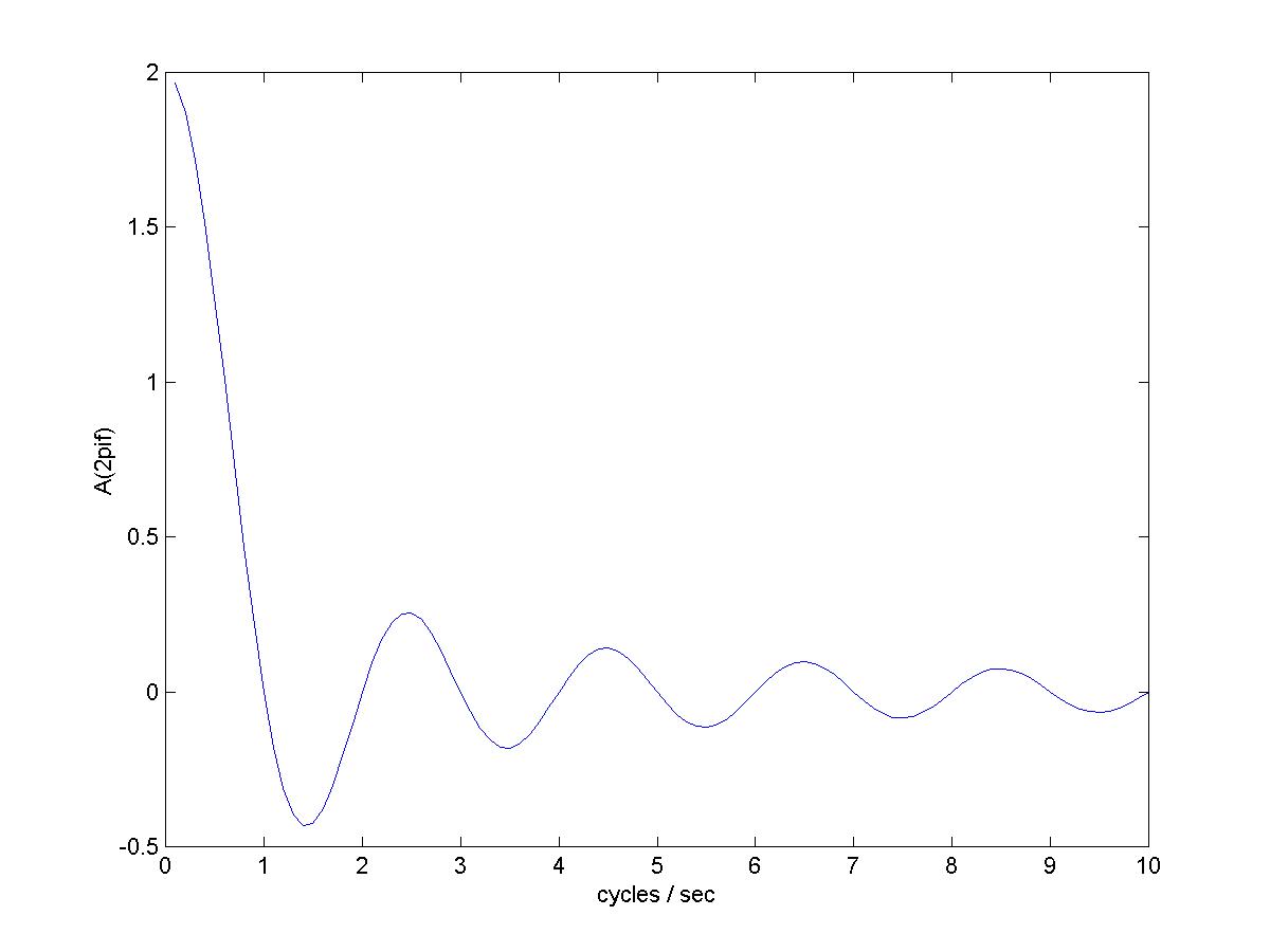 The Fourier Transform of a Pulse |
| Note that the Fourier series coefficients of a pulse train are scaled samples of the Fourier transform of a pulse | |
Impulse
Exponential
Damped oscillation
Fourier Theory using Complex Cosine-sines
We need to shift gears slightly here. Typically, a presentation of Fourier theory begins as we have begun and then at some point, 'for convenience', introduces the complex exponential form of the theory as a change in notation. The effect is to rewrite the Fourier series as a sum of complex cosine-sines. We will avoid complex exponentials, but we still need to rewrite the series as a sum of complex cosine-sines.
Why is this necessary? A sine wave is generated by a projection, say the height, of a point on a revolving wheel. But a sine wave doesn't do a good job of representing the physical process that generates it, that is, the motion of the wheel. There is a constancy to the motion of a wheel, but the sine wave speeds up and slows down. Rotation is well represented by a complex cosine-sine. By using complex cosine-sines, which initially appear more complicated, the mathematics will actually be simpler because they accurately represent the underlying process.
A Digression on Terminology - Imaginary Numbers are Neither.
Here is an apple- However if I told you that this -
  was a complex apple, and the apple on the left was the real part, and the apple on the right was the imaginary part, you'd think I was daft.
Yet, that is exactly the way 'complex numbers' are defined and constructed. Here is a number - 2343, here is a different unrelated number, 5656, and here is a complex number (2343, 5656), 2343 is the real part of the complex number, and 5656 is the imaginary part! It is impossible to overestimate the confusion this terrible terminology has caused math students at all levels.
Then the confusion is compounded by raising the irrational number e to an imaginary power i. Read that again, an irrational number raised to an imaginary power! That has got to be confusing. The notation ea+ib is ubiquitous in Fourier theory. We'll take all necessary care to avoid it.
OK, if an imaginary number is not imaginary and is not a number, what is it? An imaginary number is a type of complex number. However, a complex number is not really a number, any more than two apples are an apple. A complex number is an ordered pair of numbers. So, an 'imaginary number' is really an ordered pair of numbers where the first number is 0.
Complex Cosine-sines are the Natural Mathematical Representation for Vibration
Because -
1. they are easy to manipulate, the amplitude and phase of a complex cosine-sine can be adjusted by multiplying by a complex constant,
2. differentiation replicates complex cosine-sines, if f is damped or undamped oscillation written with a complex cosine-sine, then f ' = (σ, ω)f where σ is the damping coefficient and ω is the frequency.
Let f(t) = (cos(ωt), sin(ωt)) then f '(t) = (0, ω)f (t), that is
[cos(ωt), sin(ωt)]' = (-ωsin(ωt), ωcos(ωt))= (0, ω)(cos(ωt), sin(ωt))
Similarly for damped oscillation, if f(t) = eσt(cos(ωt), sin(ωt), then f ' = (σ, ω)f (t), that is
[eσ(cos(ωt), sin(ωt)]' = (σ, ω) * (eσ(cos(ωt), sin(ωt))
3. a complex cosine-sine fully represents the process generating the vibration.
Writing a Fourier Series as a Sum of Complex cosine-sines
We want to write a Fourier series as a sum of complex cosine-sines. The component of the Fourier series at frequency jω is (ω = 2π/T)
Ajcos(jωx) + Bjsin(jωx)
and this is the 'real' part of
(Aj, - Bj) (cos(jωx), sin(jωx))
So, we're almost there already. However, a Fourier series is a real valued function, not a complex valued function, so, we're not done. We can add a complex conjugate, and the sum of these complex cosine-sines equals the Fourier series component at frequency jω
(1/2)(Aj, - Bj) (cos(jωx), sin(jωx)) +
(1/2)(Aj, Bj) (cos(jωx), -sin(jωx))
By considering the second term above as the the contribution at the frequency -jω, we can rewrite the Fourier series as
Sn(x)=
where for j = -n, -n+1, ..... 0 ..... n-1, n
Aj = 
and
Bj = -
Similarly, we can write the Fourier transform using complex cosine-sines. Now, the value of the Fourier transform at a particular frequency is a complex number that multiplies the complex cosine-sine at that frequency in the Fourier integral. The big payoff is that the derivative rule, which follows, takes a very simple form.
The Laplace Transform
Fourier series can be used to approximate periodic functions but not aperiodic ones. Fourier integrals can be used to approximate aperiodic functions but not periodic ones. Sort of a Jack Spratt situation. We need a transform that can be used to represent both aperiodic and periodic functions. That would be the Laplace transform.
The reason that a function f(t) fails to have a Fourier transform is that the infinite integrals defining the transform don't converge. In most cases multiplying f by an exponential damping function e-αt will cause the integrals to converge and hence the Fourier transform will exist for the damped function.
So we multiply f(t) by the damping function e-αt, and take the Fourier transform of the product f(t)e-αt, and we have the Laplace transform of f(t). We don't need to prove a 'Laplace integral theorem' as it follows directly from the Fourier integral theorem. We evaluate a small set of Laplace transforms of functions that are critical in analysis and engineering, and we use this transform library in the rest of the book to solve differential equations and to analyze linear systems.
The complex valued Laplace transform is defined by
L(f)(σ, ω) = 
Laplace Transform Properties
The crucial property of the Laplace transform (it's also true for the Fourier transform) is that it transforms differentiation into multiplication by s, that is, for s = (σ ,ω)
L(f ')(s) = sL(f)(s) - f(0)
Recall the product rule for differentiation (uv)' = u'v + v'u,
integrating both sides gives
So, with u=e-σt(cos(ωt), -sin(ωt)), and dv = f ', we have u'=(-σ,-ω)u, and v=f, and

so that
L(f ')(s) = sL(f)(s) - f(0)
The key factors were the product rule for differentiation, and the property that differentiating damped oscillation results in multiplying the damped oscillation by a constant.
Examples
The Laplace transform maps the complex plane (σ ,ω) to the complex plane (a, b). A point in the domain represents the damping factor of the exponential used to modify the function, and the and frequency of the Fourier transform, a point in the range represents the Fourier transform cosine and sine components at the frequency. Thus, 'complex numbers' are being used to represent different things for the domain and range of the Laplace transform.
We can take the Laplace transform of a damped complex cosine-sine, which is easy (see the derivative of damped oscillation above):
L[e-αt(cos(βt), sin(βt))](s) = 

and this result can be used to calculate the Laplace transform of real valued damped sine and cosine waves. These are key functions in Laplace transform analysis. With this result we can identify the function generating any transform that is the ratio of two polynomials (a rational polynomial).
Laplace transform convergence
We can use MATLAB/FREEMAT to plot Laplace transform magnitudes, as shown below, this is a plot of the Laplace transform of the circuit output for the second example below
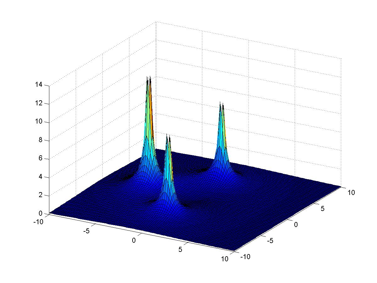
Table of Laplace Transforms
Easy integrals give a useful table of Laplace transform pairs. The CWT Laplace transform table contains only two entries! These are all you need for inverting any rational polynomial Laplace transform. The entries are
L[e-αt(cos(-βt), sin(βt))tn](s) = 1 / (s + (α, β))n
L[δ(n)(t)] = sn
Compare this to any other table of Laplace transforms! CWT is simpler, clearer, and much easier to use.
Solving Differential Equations with the Laplace Transform
We can use the Laplace transform properties and library from the previous section to solve problems where the functions involved have rational polynomial Laplace transforms. This is a wide class of problems in science and engineering. A cookbook method is given for solving them.
Algebra
We have made it through three and a half volumes with very minimal algebra, but that has to end now. Look on the bright side - finally you find out why you spent years studying polynomials in high school. The Laplace transform transforms differential equations into polynomial equations, and we'll need to solve the polynomial equations in order to solve the differential equations we started with.
We need two results, the first is the Fundamental Theorem of Algebra states that a polynomial equation of degree n has n roots (solutions) and can be written as a product of n factors of degree one.
The second result we need is that a set of n linear equations with n unknowns has a solution. This leads directly to the partial fraction expansion for a rational polynomial.
The theory has been elegant and we've obtained some amazing theorems with a modest effort. First, the bad news: the algebra required to solved even a simple problem, factoring the polynomials and writing the partial fraction expansion, however, can be intimidating. Now the good news: OCTAVE can do the algebra automatically.
A First Order System
The circuit below is like the ones we analyzed in CWT Vol. 2, with the battery replaced by a 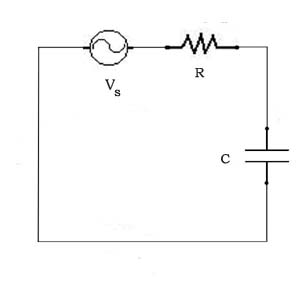 voltage generator Vs. The voltage across the resistor is i(t)R, the voltage across the capacitor is
  , and the voltage generator voltage is Vs(t). So, we have
i(t)R + + Vs(t) = 0
We'll let the voltage generator generate a unit impulse, that is, Vs(t) = δ(t), so that L(Vs) = 1.
Taking the Laplace transform of both sides of the differential equation gives
R*L(i) + (1/C)(L(i)/s) = -1
and
L(i) = -1/(R + (1/Cs)) = -Cs/(CRs + 1)
We can rewrite the right hand side,
L(i) = -1/R(CRs/(CRs + 1)) = -1/R(1 - 1/(CRs + 1))
and we can use the transform library from the previous section to write down the inverse transform of the right hand side, giving
i(t) = δ(t) + (1/RC)e-t/RC
Solution for a step input
Solution for a pulse input
Solution for a damped sine wave input
A Second Order System
Higher Order Systems
Linear Systems Analysis
The Transfer Function
Many systems can be analyzed as input/output systems, where the input is a function, always of time in our examples, and the output is also a function of time. The system is characterized by its transfer function, which is the ratio of the Laplace transform of the output to the Laplace transform of the input. Given that the system differential equation is linear with constant coefficients, the resulting transfer function is a rational polynomial, and hence invertible using our table of Laplace transforms (and a little algebra).
Block Diagrams
Given that a system, or a component of a system, can be represented by its transfer function, then we can represent the system or component by a box, and the only property of the box is its transfer function. This is a block diagram representation of the system/component. We can connect block diagrams to create larger more complex systems.
Frequency response <=> impulse response <=> transfer function
We can characterize a system by its transfer function, its impulse response, and its frequency response. The system impulse response is the inverse Fourier transform of the system frequency response. The transfer function is the Laplace transform of the system impulse response. The frequency response is transfer function evaluated at (0, ω).
The $64 Question, What Does a Pole Zero Plot Really Mean?
The transfer function of a linear system is a rational polynomial, and a rational polynomial is determined by its poles and zeros. We'll see that its possible to get from the transfer function to the poles and zeros using OCTAVE, in about as much time as it takes to type it in, and from that it is possible to write down the impulse response and step response directly, no sweat whatever (note: CWT does a way better job of facilitating this than the other books I've seen, CWT makes it COMPLETELY trivial - the CWT Laplace transform table has only 2 entries !).
Systems with Feedback
Suppose you want to design an automatic driver for a car. To make it simple we'll suppose that the car only travels in a straight line, and you only want to program point to point moves. Go to location 10 and stop. Go to location 25 and stop. And so on. Your only controls is the throttle, which we will make reversable. You could spend a lot of time trying to program the throttle controller, but even then, if you run 'open loop', without feedback, the performance of your automatic driver will probably not be very good.
To give the automatic driver any degree of accuracy, you'll need feedback, information about the actual acceleration, velocity, or position of the automobile. You'll need to incorporate this information into your control algorithm. You'll need a system with feedback.
A block diagram for a generic feedback control system is shown below. The uncontrolled plant is P. The feedback is provided by the loop back, and is compensated by H. The controller is C.
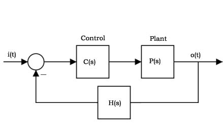
We can derive the transfer function for the overall system as follows
O(s) = P(s)C(s)(I(s) - H(s)O(s))
O(s)(1 + P(s)C(s)H(s)) = P(s)C(s)I(s)
O(s) = P(s)C(s)I(s) / (1 +P(s)C(s)H(s))
So the closed loop transfer function is
O(s)/I(s) = P(s)C(s) / (1 + P(s)C(s)H(s))
Op Amp Circuits
A PID Controller
We'll examine a system like the automatic driver described above. This is the typical servo control problem that is the basis of machine control. We'll simplify the car and throttle, so that the 'plant' is a box sliding on a table, the input to the plant is force which we control directly, and the only other force acting on the box is friction which is proportional to velocity.
A proportional, integral, derivative (PID) controller has one term which is proportional to the error signal, one that is the integral of the error, and one that is the derivative of the error. Hence its transfer function is
C(s) = Kp + Ki/s + Kds
The differential equation for the box's motion is
Mx ''(t) = f(t) - ux '(t)
So the force to motion transfer function for the box is
P(s)= X(s)/F(s) = 1/s(Ms + u)
and the transfer function for the closed loop system with a PID controller is, with H(s) = 1,
O(s)/I(s) = (Kds2 + Kps + Ki) /
((M3 + Kd + u))s2 + Kps + Ki)
Now, using OCTAVE, we can run through our repetoire of linear system analysis tools:
1 – Compute the transfer function poles and residues (partial fraction expansion)
2 – Graph the transfer function
3 – Write the equation for the impulse response
4 – Plot open and closed loop gain and phase
5 – Graph the impulse and step responses
6 – Use numerical convolution to compute the response to an arbitrary input
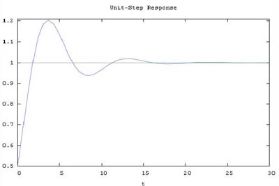
We can use the toys provided by OCTAVE/MATLAB to study the effects of the controller parameters on system responsiveness, accuracy, and stability. We can vary paramters and display the closed loop step response as easily as shown below:
 t=0:0.1:20;
M = 1;
u = 1;
Kp = 1;
Ki = 1;
Kd = 1;
num=[Kd Kp Ki];
den=[(M3 + Kd + u)) Kp Ki];
sys=tf(num,den);
step(sys,1);
title('Unit-Step Response')
The Discrete Fourier Transform and the Fast Fourier Transform
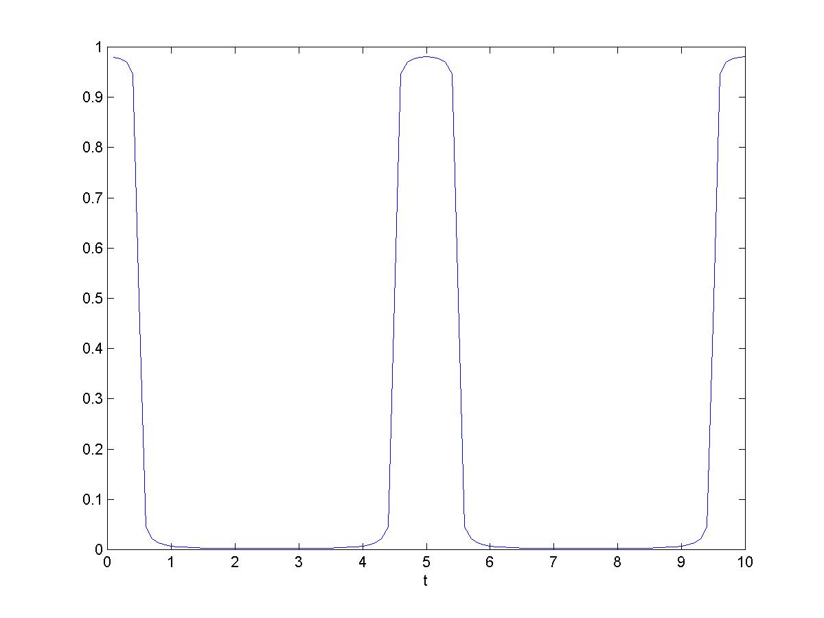
Suppose we'd like to write Fourier's score for Tchaikovsky's Overture, or ten seconds of the tune Bangarang plotted below: how can we do it? All the transforms we have seen thus far were defined by mathematical 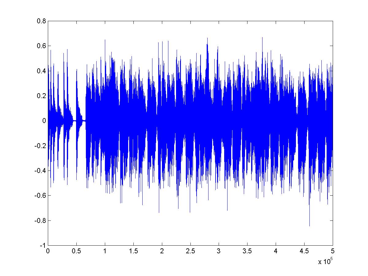 functions, and we don't have a function that calculates ten seconds of the Bangarang waveform. Instead, we have sampled data. The data for the graph was obtained by sampling microphone output at a rate of 44,100 samples per second. But, the sound amplitude was defined for every instant of the ten seconds of music, thus, there were an infinite number of possible sample values, and we only have 10*44,100, not even one percent of the total. Is that enough? (Yes, see below.)
Would you like to hear Fourier's orchestra tackle the ten seconds of Bangarang shown? Of course if we assemble the full orchestra the result will be indistinguishable from the original. So, let's limit Fourier's band to the first 25000 players (we never said Fourier's band was small). We can use the DFT described below to compute the score (the amplitude and phase of each player's note) and the result can be heard here.
The discrete Fourier transform (DFT) calculates DFT coefficients from sampled data. The formula is
Fk=
where Fk is a sequence of N DFT coefficients, and fk is a sequence of N sampled data values.
If fk is the sample sequence from ten seconds of Bangarang, then each Fk is complex, giving the amplitude and starting phase for the flute player playing at frequency k cycles per period in the Fourier orchestra's score for the ten seconds of Bangarang.
Let f(t) represent the function that was sampled. If f is band-limited, and the sampling rate high enough, then it is remarkable but true (this is proved in the book) that the DFT coefficients calculated using the sampled data are identical to Fourier series coefficients calculated by integrating f, and the original signal f(t) is recoverable from the sampled data sequence fk !
Now that the correspondence between the sampled data DFT and the Fourier series has been shown, our job is done. The DFT is an essential tool used in digital signal processing, for example, in mp3 compression. The Fast Fourier Transform (FFT) is a fast algorithm for computing the DFT.