The Physics of a Falling Apple, and a DE We Can’t Solve

According to the story, Newton discovered the Law of Universal Gravity after watching an apple fall from a tree on his country estate. Gravity is the force that pulls the apple toward the earth and causes it to fall. It also acts on the moon to hold it in its orbit.

Having discovered gravity, Newton understood that there was a force acting on the apple; now he wanted to understand the apple’s trajectory as it falls, that is, he wanted to know the position function for a falling apple. First, he needed to know how the force of gravity affects the apple's trajectory, and to this end he discovered the Second Law of Motion (after discovering the First Law of Motion), which is force (F) equals mass (M) times acceleration (A), or F = M * A.

For fun let’s use some real numbers to compute the acceleration due to gravity for an apple near the surface of the earth, the equation for the law of gravity is

F = G * M_earth * M_apple / (R * R), where

G is the gravitational constant ( = 6.67 * 10-11 m³/(kg sec2) ), this number just compensates for the units so that the answer comes out right

M_earth is the mass of the earth ( = 5.9742 * 1024 kg )

M_apple is the mass of the apple ( = 0.25 kg )

R is the distance between the centers of earth and apple ( = 6,378 * 10⁶ m ) ;

Now we can use the Second Law of Motion to compute the acceleration of a falling apple:
A = F / M_apple = (G * M_earth * M_apple / (R * R)) / M_apple = G * M_earth / (R * R)

Note that the mass of the apple divides out of the expression for A. We can use our calculators to calculate A = 10 m/sec*sec (9.8…)

Acceleration is the rate of change of velocity, so, if v(t) is the apple's velocity function, we have the differential equation
v’(t) = A = -10 (the '-' appears as the acceleration is downward)

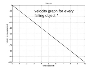
This is the type of differential equation we solved in Vol. 1, and the solution is
v(t) = -10 * t + V₀ where V₀ is the apple’s initial velocity.
The solution for V₀ = 0 is shown graphed to the left.

So, we can solve the differential equation for the apple's velocity v(t), and since p'(t) = v(t), we can write a differential equation for the apple's position function,
p'(t) = -10 * t + V₀

Can we solve this DE right now? Ans: no, solving this DE will occupy us for the remainder of Volume 2.

Graphing Solutions to DEs – Piecewise Linear Approximation

We can’t write the exact solution to p’(t) = -10 * t + 0, but we can graph an approximate solution. Suppose we 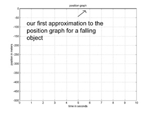want to graph the first 10 seconds of the apple’s fall. We will draw a graph made up of straight line segments (and called piecewise linear) to approximate the apple’s position function. How to do it? We'll start with a single segment for the entire 10 seconds. The apple’s starting altitude is 0, so, now, all we need is the slope of the line. We know the apple’s velocity at time t = 0 is 0 (m/sec), and its velocity at time t=10 is –100. So, we could use an ‘average’ velocity, but, let’s do the least amount of work possible, and just use the velocity at the start of the interval, v(0) = 0, so that our first approximation is a horizontal line at altitude 0. This gives us the linear graph shown to the left.

A lousy approximation to the true trajectory of a falling apple, but, hey, we're just getting started.

Now, notice what happens when we divide the 10 seconds into two 5 second intervals and use a linear 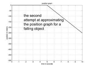approximation for each subinterval. We get the same graph for the first 5 seconds. At t=5 our approximate solution is still at altitude 0, so the solution for the second interval starts at 0, and the slope of the solution is given by the velocity at the start of the second 5 seconds, which is v(5) = -50, giving the piecewise linear graph to the left.

Not a good approximation, but a lot better than our first one.

If we divide the 10 seconds into 10 one second intervals, and follow the method used above to produce a linear approximation for each 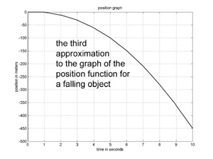subinterval, we get the graph to the left. This is a pretty good approximation to the true solution to the DE. Compare it to the exact solution below.

This is the technique engineers most often use to solve differential equations! It’s just this simple, and it can be used to obtain a solution to any DE.

Defining 'Instantaneous Velocity' and Differentiating t²

In Volume 1, we learned that the velocity function for p(t) = V * t + P₀ is p’(t) = V. We were a bit cavalier there, not really bothering with definitions, and when velocity is not constant we need to be more careful. The velocity function p’(t) calculates the runner’s velocity at the instant when time equals t – what does that mean? Here is the problem: the formula that calculates velocity for the interval t₁ to t₂ is velocity = distance / (t₂ – t₁). This formula is more than a way of calculating velocity, it is the definition of velocity. And, it works fine for intervals, but not for instants. Why not? For an instant at time t, t₁ = t and t₂ = t, so, the formula becomes distance / (t₂ – t₁) = 0/0. This is a bit of a sticky wicket.

With this difficulty in mind, let’s set out to define and calculate the velocity for p(t) = t², plotted 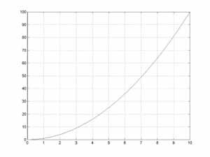to the left. What is the velocity at time t=4, for example? Intuitively, we can approximate the velocity at the instant t=4 by calculating the velocity for a short interval starting at 4. The distance traveled in the interval 4 to 4 + h is given by
p(4+h) – p(4) = (4+h)² - 4² = 4² + 2*4*h + h² - 4² = 2*4*h + h²
and the for velocity for the interval (velocity = distance / time) is
(2*4*h + h²) / h = 2 * 4 + h
As h becomes smaller, the approximation improves, and the velocity for the interval approaches 2*4. We define the instantaneous velocity of any function at time t to be the limit of the velocity for a interval of length h starting at time t, as h approaches 0. So, we see that p’(4) = 2*4 = 8.

For any value of t, the distance traveled for the interval t to t+h is given by
p(t+h) – p(t) = (t+h)² - t² = 4t² + 2*t*h + h² - t² = 2*t*h + h²
and hence the velocity is
(2*t*h + h²) / h = 2 * t + h
As h becomes smaller, the velocity for the interval approaches 2*t, and thus we have
p’(t) = 2*t

That's the crux of calculus right there, folks.

Integrating p’(t) = A * t

We can integrate linear functions geometrically using triangles. This is a bit of a makework chapter, the real next step in integration is the Fundamental Theorem of Calculus covered in Vol. 3

Given the position function p(t) = A*t² / 2 and the velocity function p'(t) = A*t, we will evaluate the integral
The area corresponding to the integral is shown shaded in the figure below. 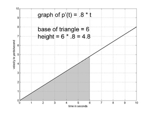We will evaluate the integral geometrically.

The formula for the area of a triangle is one-half the base times the height. The area under the graph of A*t for the interval 0 to t₂ is (1/2) * t₂ * (A* t₂) = A* t₂² / 2.

We can calculate the area under the graph for the interval t₁ to t₂ by subtracting the area of the smaller triangle from the area of the larger triangle, 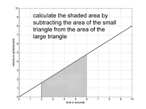giving A* t₂² / 2 – A* t₁² / 2.

Recall that the Fundamental Theorem of Calculus states that
= p(t₂) – p(t₁)
The calculation above shows that the FTOC is true when p(t) = A*t² / 2 and p'(t) = A*t.

The Trajectory of a Falling Object – Solving the Differential Equation F = M * A when F is the Force of Gravity

We can differentiate p(t) = A*t²/2 + V₀*t + P₀ by adding the derivatives of each term, giving p’(t) = A*t + V₀ + 0. Then, differentiating p’(t) gives p’’(t) = A.

So, if A = -10, then apparently p(t) is a solution to the DE p’’(t) = -10 for every value of P₀ and every value of V₀. Thus we have solved the DE that characterizes the trajectory of a falling object, that is p’’(t) = -10. The method used was 'by inspection', that is, we looked at the DE and recognized that we could immediately write down a solution.

The initial position of the trajectory defined by p(t) = A*t²/2 + V₀*t + P₀ is p(0) = P₀ and the initial velocity is p'(0) = V₀. We can choose these constants to fit the physical system being modeled as shown below.

If an 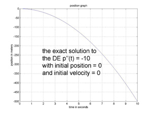apple falls from an initial altitude of 0 meters, then its initial position P₀ is 0, its initial velocity V₀ is 0, and its trajectory is given by p(t) = -5*t²

If an apple is thrown upwards from an 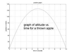initial altitude of 0 meters, with an initial upward velocity of 50 meters/sec, then P₀ = 0, V₀ = 50, and its trajectory is given by p(t) = -5*t² + 50*t + 0.

Air resistance opposes the flight of any object near the earth, and is proportional to the square of the velocity. If we include drag in the differential equation for the trajectory of a falling apple we have A – D* p’(t) * p’(t) = p’’(t) where D is the ‘drag coefficient’ of the apple. This DE is difficult to solve analytically (that is, with a mathematical expression for p), however, we can easily determine a graphical solution using the method of piecewise linear approximation discussed above (as shown in the book).

Electrical Circuits

We can analyze electrical components and simple circuits just by changing the names of the functions, the math is the same.

Kirchoff's Law states that the sum of the voltages around a loop is zero, so, for the circuit below we have
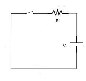0 = v_C(t) + v_R(t)
where v_C is the voltage across the capacitor and v_R is the voltage across the resistor. Differentiating both sides gives
0 = v_C'(t) + v_R'(t)
The rate of charge for a capacitor is v_C'(t) = i(t)/C where i is the current through the capacitor, and v_R'(t) = Ri'(t), so that when the switch is closed the current in the circuit satisfies the DE
0 = i(t)/C + Ri'(t)
An innocuous enough looking DE, but the solution requires the exponential function (one of nature's favorites), so an analytical solution is deferred to Vol. 3. The important thing is to see how DE's are used to model physical systems, and we do compute numerical solutions, using the method of Chapter 2, for various simple circuits.