Motivating the Secondary School and Undergraduate Math Curriculum

The only way to motivate the mathematics curriculum is to model and analyze interesting physical phenomena. Two typeof physical systems are studied in the CWT series, mechanical and electrical. In this page we extend the examples in the CWT series to two dimensional orbits (not possible in the books because trigonometry is required).

The Equation that Characterizes the Trajectory of a Falling Object

First, the math - the force of gravity F on an object of mass m near earth is given by

where G is the gravitational constant, m_E the mass of the earth, R the distance between the centers of the earth and the object, and the minus sign is there because the force is downward.

Newton's 2nd Law of Motion tells us how the force of gravity affects a falling object,

which states that if a force F acts on an object of mass m then the objects accelerates, with the acceleration A equal to F/m.

Combining the equations above gives the equation for the acceleration of a falling object

Orbits are two dimensional, and in two dimensions it's necessary to resolve forces and accelerations into their x and y components. If the magnitude of the force of gravity on an object at coordinates (x,y) is g, then the x component of gravity is g*cos(a) = g*x/R and the y component is g*sin(a) = g*y/R where (R, a) are the polar coordinates of (x,y).

That's it for the math.

Computational Calculus, i.e. Using MATLAB/FREEMAT/OCTAVE to Calculate Orbits

We will model a falling object above the earth. The coordinates of the center of the earth are (0,0), and the coordinates of the object are (x,y). We will model a trajectory of duration T seconds and divide it into N subintervals, numbered 1 to N, of lenght dt = T/N. As the trajectory is computed we'll keep lists (i.e. MATLAB vectors) of the time, the x and y positions, and the x and y velocities at the start of each subinterval, in vectors named t, x, y, vx, and vy respectively.

The basis of the model is the code that advances time, position, and velocity from the start of one subinterval to the start of the next next. It is given below.
for i = 2,N+1                              % perform the calculations for subintervals 2 thru N+1
     t = t + dt;                              % time at start of interval i
     x(i)=x(i-1)+vy(i-1)*dt;                    % x position at start of interval i
     y(i)=y(i-1)+vy(i-1)*dt;                    % y position at start of interval i
     r = sqrt(x(i-1)^2 + y(i-1)^2);          % r at start of interval i-1
     g = -G*mEarth /r^2;                        % magnitude of gravity acceleration at start of interval i-1
     ax = g*x(i-1)/r;                        % resolve gravity acceleration into x and y components
     ay = g*y(i-1)/r;                        %
     vx(i) = vx(i-1)+ ax*dt;          % x velocity at the start of the ith interval
     vy(i) = vy(i-1)+ ay*dt;          % y velocity at the start of the ith interval
end                              % end of loop
and the rest is bookkeeping. We'll refer to the code above as the BASIC LOOP

The Space Station Orbit

The BASIC LOOP code determines the trajectory of the orbit once the initial position and velocity are given. So, to simulate a satellite in low earth orbit we only have to provide the initial position and velocity and start the program. 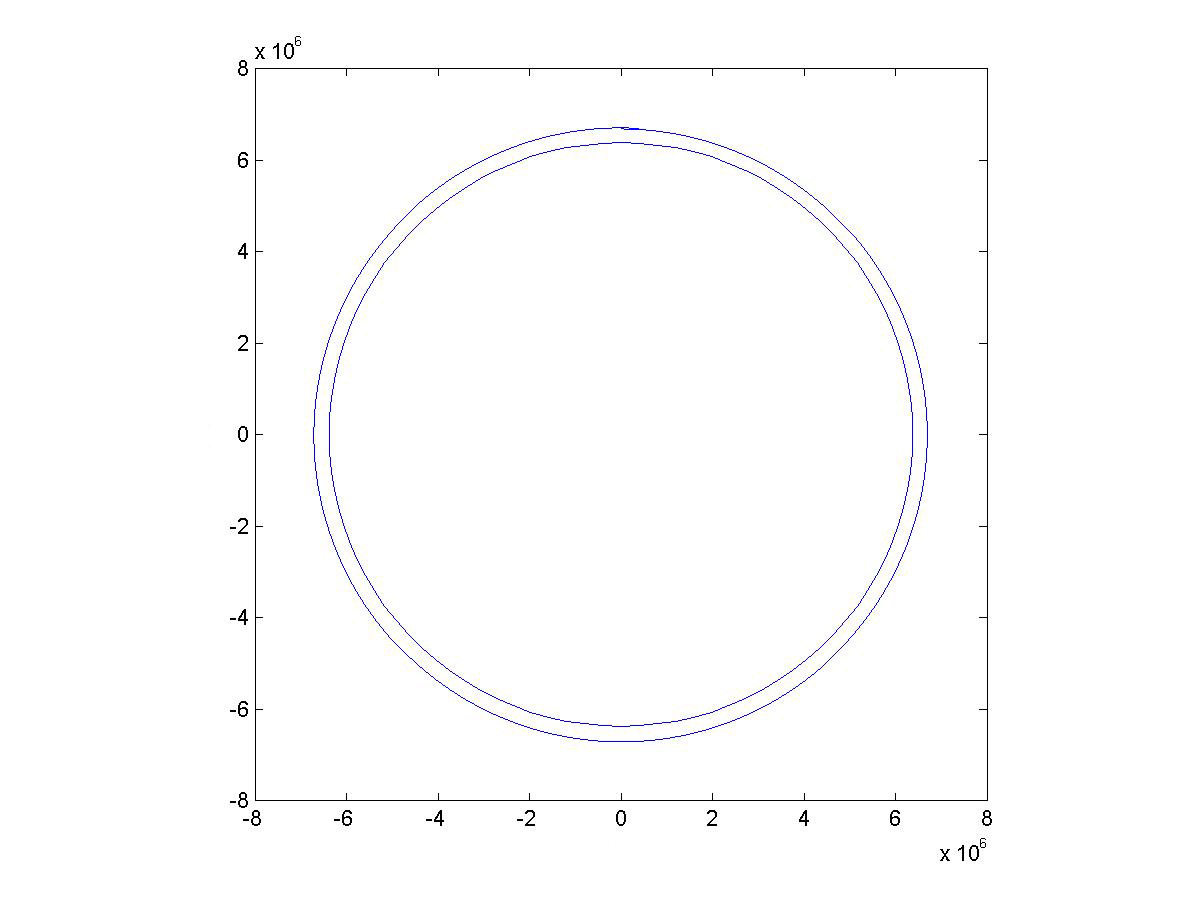We'll start the satellite at 300 km above the north pole, with an initial velocity of 77502 m/s determined purely by trial and error to get an approximately circular orbit. The code for the simulation is as follows:

t=0;             % start at time t = 0
N=5000;           % compute trajectory for 5000 seconds
dt=1;           % each subinterval has length = 1 second
x(1)=0;           % initial x position
y(1)=300000;           % initial y position
vx(1)=77502;           % initial x velocity
vy(1)=0;           % initial y velocity
BASIC LOOP
plot(x,y)           % draw the orbit

The graph shows the calculated orbit and the outline of the earth for reference. The code for drawing the earth is:
hold on           % this holds the orbit graph
for i=1:101           % here we create a circle corresponding to the earth's outline
   xE(i)= rEarth*cos(2*pi*i/100);           % x coordinate
   yE(i)= rEarth*sin(2*pi*i/100);           % y coordinate
end           %
plot(xE,yE)           % draw earth's outline
We'll refer to this code as DRAW EARTH.

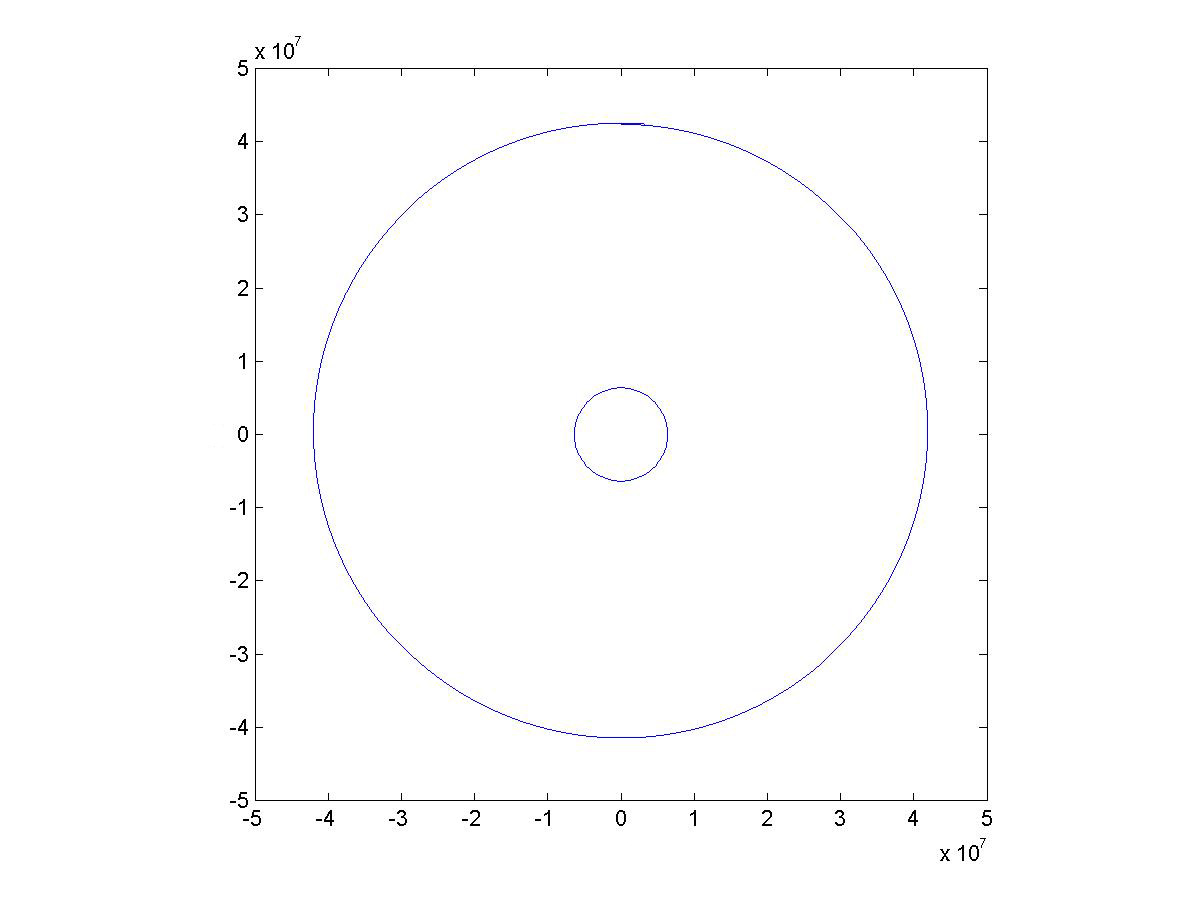
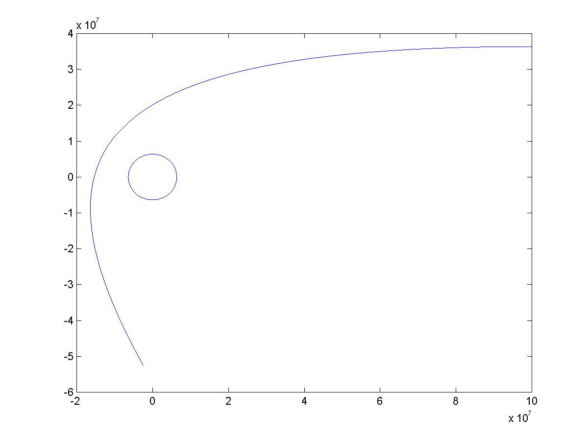
A Geosynchronous Orbit

The figure shows a geostationary orbit at 36000km. A geostationary orbit is a circular orbit above the equator, with a period of one day. Thus a satellite in a geostationary orbit appears to a ground observer to be in a fixed position in the sky. The code for the simulation is as follows: The code for the simulation is as follows:
t=0           % start at time t = 0
N=5000           % compute trajectory for 5000 seconds
dt=1;           % each subinterval has length = 1 second
x(1)=0;           % initial x position
y(1)=36000000;           % initial y position
vx(1)=3055;           % initial x velocity (determined by trial and error)
vy(1)=0;           % initial y velocity
BASIC LOOP
plot(x,y)           % draw the orbit
DRAW EARTH

An Asteroid Fly By

The figure shows an asteroid fly-by with a parabolic orbit. The code for the simulation is as follows:
The code for the simulation is as follows:
t=0           % start at time t = 0
N=5000           % compute trajectory for 5000 seconds
dt=1;           % each subinterval has length = 1 second
x(1)=100000000;           % initial x position somewhere out in space
y(1)=30000000;           % initial y position somewhere out in space
vx(1)=-3000;           % initial x velocity, speeding toward earth
vy(1)=0;           % initial y velocity
BASIC LOOP
plot(x,y)           % draw the orbit
DRAW EARTH

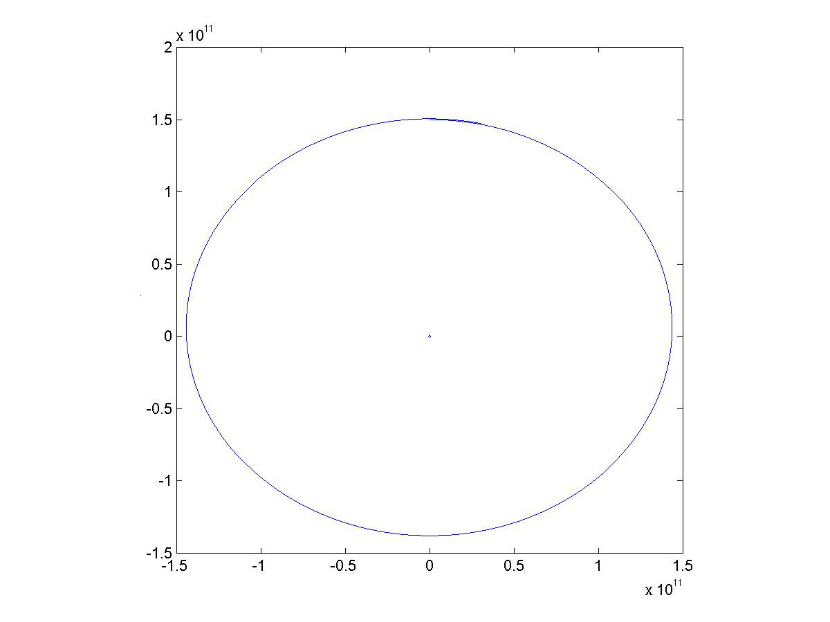
The Earth's Orbit Around the Sun

The BASIC LOOP code can be modified to calculate orbits around the sun by replacing the mass of the earth (the constant mEarth in the code) with the mass of the sun (mSun). The mass of the sun is 1.98892 × 10³⁰kg, the earth’s orbit around the sun is an ellipse with a semi-major axis of 150,000,000km, the sun’s radius is 695500km. The period of the earth’s orbit is one year. Using these numbers produces an approximation to the earth’s orbit around the sun as shown in the figure. The code for the simulation is as follows: The code for the simulation is as follows:
t=0           % start at time t = 0
N=365*24*60*60           % compute trajectory for one year
dt=1;           % each subinterval has length = 1 second
x(1)=-150000000000;           % initial x position
y(1)=0;                              % initial y position
vx(1)=-3000;           % initial x velocity, speeding toward earth
vy(1)=28500;           % initial y velocity
BASIC LOOP (with mEarth replaced by mSun)
plot(x,y)           % draw the orbit
DRAW SUN (DRAW EARTH with rEarth replaced by rSun)

Atmospheric Drag and Terminal Velocity

An object falling close to the earth is also acted on by the force of atmospheric drag. One model of the drag force is given by the equation
   F_d = p*v²*C_D*A/2
where F_d is the magnitude of the drag force, p is atomspheric density, v is the object's velocity, C_D is the object's coefficient of drag, and A is the object's cross sectional area. The direction of the drag force is opposite to the direction of the velocity.

Amospheric density is 1.3 kg/m3 at sea level to falls to 0 at altitude 35 km and above. We implement a simple linear 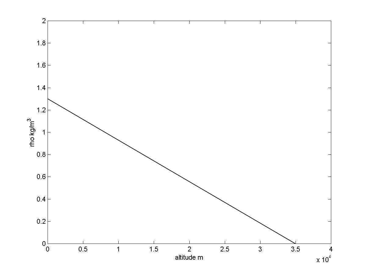model of atmospheric density shown in the graph.

Atmospheric density is computed by the following code:
if (r(i-1) - rEarth > 35000) p = 0           % density is 0 if altitude > 35000 m
else p=1.3*(1-p(i)/35000);           % compute air density for altitude <= 35000
endif

The drag force is computed and resolved into its x and y components with the following code:
v = sqrt(vx(i-1)^2 + vy(i-1)^2);           % compute velocity magnitude
fd = p*v^2*Cd*A/2'           % compute drag force magnitude, note: requires values for Cd and A
dax = -F/m * vx(i-1)/v;           % compute drag accreleration and resolve into x and y components
day = -F/m * vy(i-1)/v;

The code can be inserted into the BASIC LOOP, and the drag acceleration added to the gravitational acceleration, to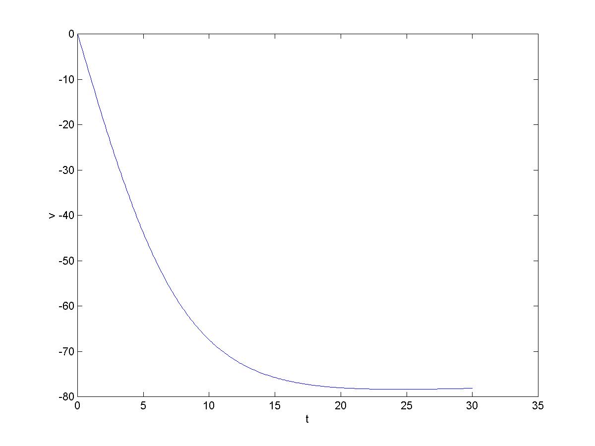
incorporate atmospheric drag into the model. The graph shows the result of dropping an apple from a height of 2000m and using the values C_D=0.5, A=.0025m², and m_Apple=0.5kg, and modifying the BASIC LOOP as above produces the velocity shown. Note that the ‘terminal’ velocity is reached after about 23 seconds and then increases (becomes less negative) slightly due to increasing air density. The code for the simulation is:
t = 0;
N = 100;
dt = 1;
x = 0;
y = rEarth + 2000;
vx = 0;
vy = 0;
BASIC LOOP (with atmospheric drag model added)
plot(vy)

The Juno Space Probe

The US launched a probe to Jupiter on Aug. 5, 2011. The trip to Jupiter will take five years, and utilizes a slingshot, or gravity assist, trajectory. The boost rocket put a Centaur upper stage and the Jupiter probe into a low 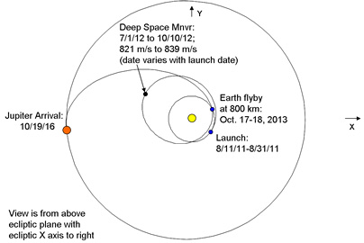orbit around the earth. The Centaur then launched the probe into a deep space orbit around the sun that will return to the earth in two years! The gravitational field of the earth will then accelerate the probe and send it on its way to Jupiter. The flight of the probe is un-powered except for two deep space maneuvers a year into the flight. A diagram of the actual planned trajectory is shown in the figure.

It’s helpful to see an animation to understand how the slingshot works, and that can be seen here
http://www.youtube.com/watch?v=sYp5p2oL51g

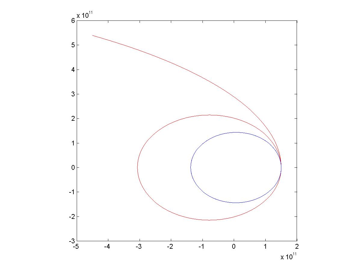
Once the probe detaches from the Centaur booster it is acted on only by the gravitational fields of the earth and the sun (except for the two deep space maneuvers which we will not model). In an example above we computed the earth's orbit around the sun. We will also need to compute the probe's trajectory. The forces acting on the probe are the gravitational force of the sun on the probe and the gravitational force of the earth on the probe.

The variables x, y, vx, and vy will store the position and velocity of the earth relative to the sun. We'll add variables xp, yp, vxp, and vyp, to store the position and velocity of the probe relative to the sun. The gravitational force of the sun on the probe and the resulting acceleration is calculated by:
rp = sqrt(xp(i-1)^2 + (yp(i-1)^2);           % the sun to probe distance
apx = -(G*mSun/rp^2) * xp(i-1)/rp;           % compute acceleration due to sun's gravity and resolve into x and y components
apy = -(G*mSun/rp^2) * yp(i-1)/rp;

The gravitational force of the earth on the probe and the total probe acceleration is calculated by:
rpe = sqrt((xp(i-1) - x)^2 + (yp(i-1)- y)^2);            % the earth to probe distance
apx = apx -(G*mEarth/rpe^2) * (xp(i-1) - x(i-1))/rpe;            % compute x component of acceleration due to earths's gravity add to acceleration due to sun
apy = apy -(G*mSun/rp^2) * (yp(i-1) - y(i-1))/rpe;            % compute y component of acceleration due to earths's gravity add to acceleration due to sun
px(i) = px(i-1) + dt*vpx(i-1);           % advance probe position and velocity
py(i) = py(i-1) + dt*vpy(i-1);
vpx(i) = vpx(i-1) + dt*apx;
vpy(i) = vpy(i-1) + dt*apy;

Once the probe is launched from the Centaur, and minus the mid-course maneuvers of the actual probe, the trajectory of the probe is completely determined by the gravitational forces of the sun and earth acting on the probe, and the code above accounts for those forces, so with it added to the BASIC LOOP we are good to go. The only thing required is to tweak the initial conditions so that when the probe returns to its approximate launch point, two years into the mission, it comes in behind the earth and gets close enough to the earth so that the earth's gravitational force accelerates it into the Jupiter bound orbit. We did that, and the results are shown:
dt=2;            % dt = 2 seconds
N=3*365*60*60*24 / 2;            % run the simulation for 3 years
x=-rEarthOrbit;            % initial position of earth relative to the sun
font color=green>y=0;
vx=0;            % initialize earth orbit velocity
vy=-28500;
xp=-rEarthOrbit - rEarth - 200000;           % launch the probe from an orbit of 200km above earth
yp=0;
vxp=0;           % the probe launch velocity was determined purely by trial and error
vyp=-28500 - 5265;
BASIC LOOP modified with code above
plot(x,y)           % print earth orbit
hold on           % hold graph
plot(xp,yp)           % print probe orbit

The earth and probe orbits can also be displayed in 3-d using the plot3 command, as shown in the figure. The code required is
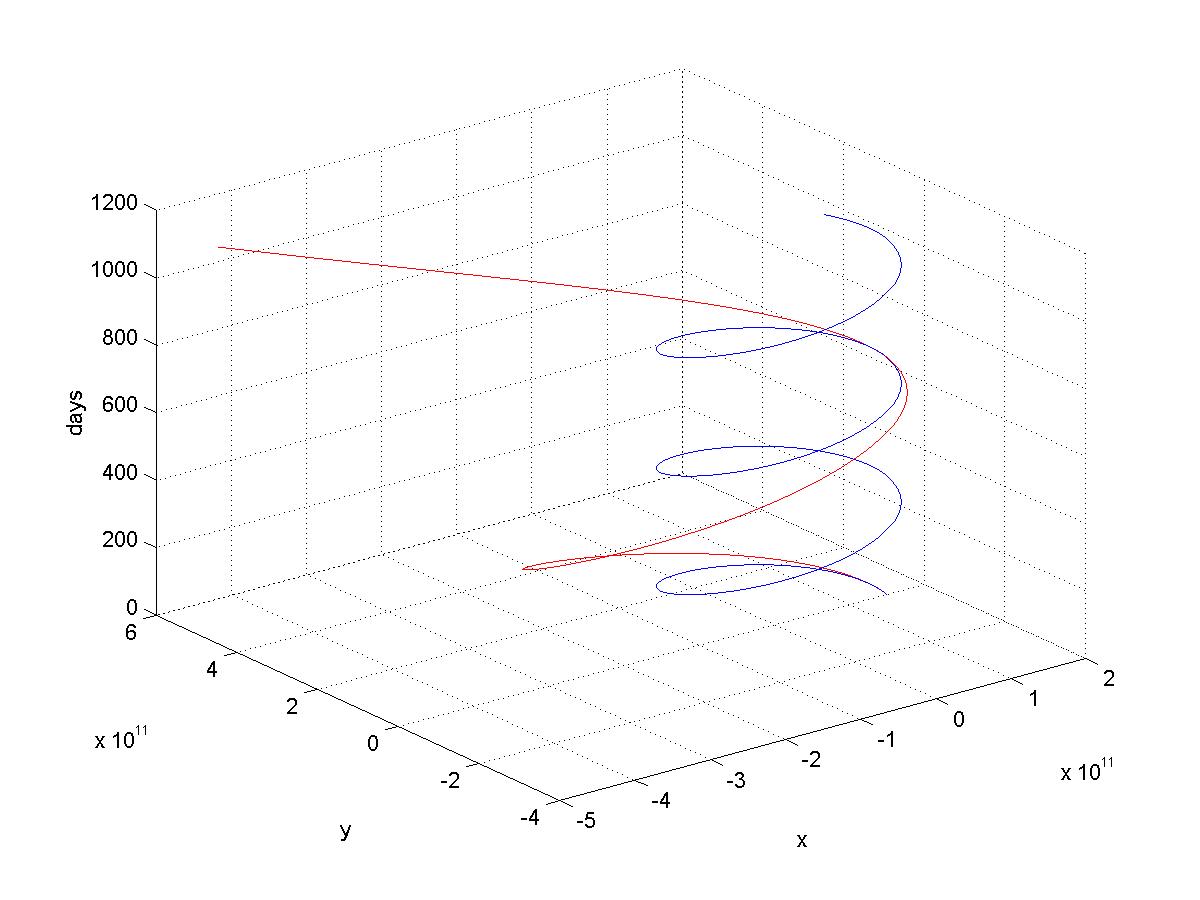
t=dt*([1 : N] - 1);           % generate the time index
plot3(x,y,t,'r')           % print earth orbit in red
hold on           % hold graph
plot3(xp,yp,t)           % print probe orbit