Introduction

Analytical calculus, the calculus that Newton discovered, can be difficult. Computational calculus, the calculus that engineers use today, is always easy. We'll demonstrate this by solving the world's first differential equation, the equation for the trajectory of a falling apple, both ways.

The Equation that Characterizes the Trajectory of a Falling Object

Newton began by discovering gravity, the force of gravity F on an object of mass m near earth is given by

where G is the gravitational constant (a number that adjusts for the force, mass and length units, different units require a different constant), m_E the mass of the earth, R the distance between the centers of the earth and the object, and the minus sign is there because the force is downward.

Then Newton discovered the laws of motion. The second law of motion is

which states that if a force F acts on an object of mass m then the objects accelerates, with the acceleration A equal to F/m.

Combining the equations above gives the (differential .... shhh, don't tell) equation for the acceleration of a falling object

The discovery of gravity and the laws of motion were huge conceptual and pivotal breakthroughs in the history of science. But, to this point the math involved has been nothing beyond multiplication and division.

Computing the Trajectory of a Falling Object

Can we compute the trajectory of a falling object, an apple say, with no more math than addition, multiplication and division? Yes we can, no problem.

The only math in this, the computational section is ..... if you drive at 5 mph for one half hour, how far have you gone? ... ! Computational calculus reduces to this equation, distance equals velocity times time !!!!!

We know the intial distance, when the apple starts falling, between the center of the earth and the center of the apple, call it r₁. We know the intial velocity of the apple, it's at rest the instant we drop it, so its initial velocity, call it v₁, is 0. And we are able to compute the initial acceleration of the apple, call it A₁ from the equation above A₁ = -Gm_E/r₁².

So, we know the initial position r₁, and we know the apple's initial velocity v₁=0 for a dropped apple, so the apple's position at time t is its initial position (r₁) plus the distance it travels (velocity times time), that is r₁ + 0 * t = r₁ . Oops, the apple doesn't seem to be falling at all. Our formula has failed us, because after an apple is dropped it accelerates and its velocity changes, and the formula only works for constant velocity motion. What to do? Not to worry, we can still use our formula, because we have a trick up our sleeve.

Here is the trick, we'll divide the time interval of the trajectory into short subintervals. We'll start with the first subinterval and compute the trajectory for that subinterval using our formula distance equals velocity times time. From that computation we'll know the position and velocity at the start of the next subinterval, and we'll repeat the process, for all the subintervals.

Here's how we'll do it: let r_i be the apple's position at the start of the i^th subinterval, v_i the apple's velocity at the start of the i^th subinterval, A_i the apple's accceleration at the start of the i^th subinterval, and dt the length of each subinterval: then we compute as follows -
1. the apple's position at the end of the i^th subinterval is r_i+1 = r_i + v_i*dt
2. the apple's velocity at the end of the i^th subinterval is v_i+1 = v_i + A_i*dt = v_i - Gm_E/r_i²*dt
The position and velocity at the end of the i^th subinterval are the position and velocity at the beginning of the i+1^st subinterval, so now we're ready to go to the i+1^st subinterval.

Let's do a few steps of an example, with, as is always our wont, easy numbers. Suppose we want to determine the 10 second trajectory of a falling apple. If we use real numbers we'll be in big trouble because G is very small (6.7*10^-11N(m/kg)²) and m_E and r are very large (5*10²⁴m and 6*10⁶m) and the calculations will be all but impossible by hand, so we'll choose new numbers to make the example illustrative and easy to calculate. We'll start with r₁ = 10, v₁ = 0, and Gm_E = 20, and the subinterval length will be 5 seconds ... hey, I said the numbers would be easy.

We begin with the first subinterval:
r₂ = r₁ + v₁*5 = 10 + 0*5 = 10
v₂ = v₁ + A₁*5 = 0 - 20/10²*5 = -1        Note: A₁ = -Gm_E/r₁²
the second subinterval:
r₃ = r₂ + v₂*1 = 10 - 1*5 = 5
v₃ = v₂ + A₂*1 = -1 - 20/10²*5 = -2       Note: A₂ = -Gm_E/r₂²
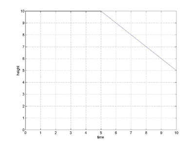
The graph of the trajectory is plotted to the left.

Note: r₁ is the position at time t=0, r₂ is the computed position at time t=5, r₃ is the computed position at time t=10

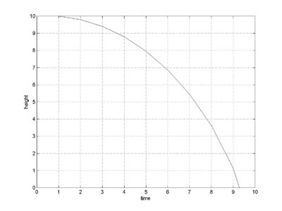
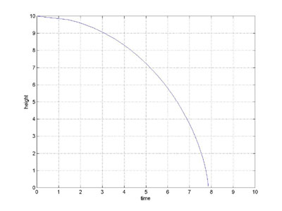
Notice that the ball doesn't fall at all for the first subinterval of 5 seconds (r₁=10 and r₂=10), it just remains motionless, and then falls at a constant velocity for the second 5 second subinterval. That doesn't look much like the real trajectory of a falling apple. Again, not to worry, the problem is that the step size is too big. If we reduce the step size to 1, we get the following graph (the MATLAB program that computed the graph is also shown)

    r(1) = 10; t(1) = 0; v(1) = 0;      
    Gme = 20;
    dt = 1;       % the subinterval time, 1 second
    for i=2:11      
        t(i) = t(i-1) + dt;      % calculate start time of subinterval i
        r(i) = r(i-1) + v(i-1)*dt;    % calculate position at start of subinterval i
        a = -Gme/r(i-1)^2;      % calculate acceleration for subinterval i-1
        v(i) = v(i-1) + a*dt;      % calculate velocity at start of subinterval i
    end
    plot(t,r)      % plot the graph
    xlabel('time')      % label the graph
    ylabel('height')

That's more like it.

The calculations above assume that velocity and accerleration are constant for each subinterval, and these assumptions introduce errors into the trajectory but they are inconsequential if the subintervals are small enough. The only difficulty is that small subintervals require a lot of computations. But hey, that's what computers are for.

So far, no math beyond addition, multipication and division, and the division was required by the acceleration formula, not the calculus.

Finding the Trajectory of a Falling Object Analytically

Newton's objective was to find the trajectory of a falling apple, and as we've seen this can be done with no more math than addition, multiplication and division, so why did Newton develop calculus? Well, surprise, we've been doing calculus. We've computed the solution to a differential equation, and solving differential equations is the sine qua non of calculus. And the only math we've used is addition, multiplication, and division. We call this computational calculus.

Newton' problem was that he didn't have a computer to perform the millions of calculations needed to compute the trajectories of the apple, the moon, the planets, etc. So, by necessity Newton had to solve the problem in a way that did not require millions of calculations. In two dimensions this problem is the two-body problem and the solution is given on the Planetary Motion page linked to the left. Here we'll use the standard CWT approach of reducing the number of dimensions to the minimum, to attempt to simplify the problem. So we have the differential equation A = -g/r*2 where g = GMe and is constant. In the standard notation, we have

We can begin to get to a solution by multiplying both sides of the equation by r'(t), giving

Both sides of this equation can be integrated, giving

thus

and solving for r'(t) gives

Treating r as a variable, we have

Integrating both sides of the second equation gives

Where D is a constant of integration. That's a formidable equation, and I integrated the function, i.e. obtained this formula, using Mathmatica's symbolic integrator. We could now verify that the integral is correct by differentiating the right hand side, and I estimate that would take a page of algebra and calculus. We'll leave it as an excercise for the skeptical reader.

Our goal is to determine r as a function of t, and what we have is t as a function of r. We could use this function in an iterative procedure to estimate r as a function of t but we'll forgo that exercise.

We can plot r as a function of t, and turn the graph on its side, which shows a graph of r versus t, as shown below

The Verdict

The development of the computational solution is complete, transparent, and all on the page. It is easy to understand right now (note: it may require a little patience), even if you've never studied calculus at all. There is no more theory to understand, this is it !

The development of the analytic solution however, is just an outline. It relies on concepts, theorems, derivations, and theory that is assumed to be known to the reader. Even given the theoretical framework, many details are left out (e.g. the integral derived by Mathematica). It is difficult to understand even if you've had several calculus courses. This solution to the falling object problem is NEVER presented in calculus or physics courses, because it is too difficult. Instead the problem is simplified by assuming that the force of gravity is constant over the entire trajectory, which makes for an easy analytic solution.

Both methods accomplish the same objective, they obtain a solution to the differential equation.

The problem solved above was expressed analytically, that is, gravity was modeled by a simple analytic function. In the real world of flight and orbit determination that model is not sufficiently accurate (as the earth is not a perfect sphere of uniform density), and more accurate and complex models must be used. The most accurate models of earth's gravity are determined empirically by measurement and cannot be represented by a formula, even a very complex formula. So, in the real world, it is often not possible to even express problems of interest analytically, much less solve them analytically. However, the computational approach to solving a differential equation is perfectly happy with computational models, of gravity for example, and hence is the only way these problems can be solved.

Sales Pitch

Calculus Without Tears is the only calculus method that begins with computational calculus. This gives the student immediate access to the methods of modeling and solving problems in mechanics, electrical circuits, and other branches of physics. Also, it provides a conceptual basis for learning analytical calculus. Each method of analytical calculus becomes a technique for achieving already understood goals, instead of a potential gordian knot that is necessary to unravel in order in order to advance to the next step and to avoid the collapse of the whole edifice.