
Calculus Without Tears
Maxwell's Equations
Introduction
Mankind's first great mystery was understanding the motion of objects in the sky. Solved by Newton. The second great mystery was understanding light. Solved by Maxwell. Maxwell's four equations explain all electrical and magnetic phenomena, as well as electromagnetic radiation, which includes light.
The equations follow directly from the analysis of simple experiments. We'll briefly review the experiments and the equations that summarize their results.
Maxwell added one term to one equation, totalling (depending on the notation) maybe 5 keystrokes. We'll see how Maxwell's term leads to the wave equation for electromagnetic radiation. Maxwell noticed that the calculated velocity of electromagnetic radiation closely matched the experimentally determined speed of light. Mystery solved.
Coulomb, Faraday, and Ampere's Equations, from the Experimental Results
Maxwell's four equations correspond to four electro-magnetic laws that had already been discovered by others. Maxwell cast the laws in a uniform terminology and added one term to one of the laws. First, we will look at the four laws without Maxwell's addition. Each of these laws follows directly from experimental results without the need for any elaborate mental gymnastics.
Equation 1 - Coulomb's Law of Force
The early Greeks noticed that when a rod of amber (Greek word: electron) was rubbed with fur it would then attract small bits of paper or other light materials. Experiments with static electricity continued through the centuries, and were finally quantified by Coulomb in the eighteenth century. When amber is rubbed with fur it acquires an excess negative charge; if the amber then touches a small bit of paper some of the negative charge will be transferred to the paper. When glass is rubbed with silk it acquires an excess positive charge; if the glass then touches a small bit of paper some of the positive charge will be transferred to the paper. Coulomb did these experiments and measured the forces between the bits of paper. He observed that like charges repel, and unlike charges attract, and he summarized his results in Coulomb's Law of Force, which states that the force between two electrically charged objects is given by
F = (1/4πe0)·(Q1·Q2/R2)
where e0 is a constant, the 'permittivity of free space',
Q1 is the charge on one of the objects,
Q2 is the charge on the other object, and
R is the distance between the objects.
Coulomb's Law of Force looks just like Newton's Law of Gravity, so, I don't imagine Coulomb had to rack his brain for too long to come up with it.
Coulomb's Law of Force tells us everything there is to know about charged particles at rest. If electrons didn't move, very rapidly, we'd be done. When charged particles do move rapidly, magnetic fields are created, and we have the next three equations.
Vector Fields
One way of looking at Coulomb's Law of Force is to imagine an electric force field that surrounds a charged object. That is, at each point in the space surrounding a charged object there is a vector E(x,y,z) = (Ex(x,y,z), Ey(x,y,z), Ez(x,y,z)) having the direction and magnitude of the force the object would produce on an object, with charge Q = 1 coulomb, located at (x,y,z).
A 'vector field' is a function giving a vector for each point in space, like E(x,y,z) above. Does this force field 'really exist', or is it just a mathematical artifice? Stay tuned.
The force field of a single charged particle radiates straight outward from the particle.
 When there is more than one charged particle, the electric field at a point is found by summing the electric field vectors of each of the particles, as shown in the diagram.
Equation 2 - There Are No Magnetic Monopoles
Experiments continued in generating static electricity from the time of the Greeks . In the eighteenth century the Leyden jar was developed, this device could hold a large static charge that could subsequently be discharged creating sparks and other effects. Near the end of the 18th century, the Italian Galvani touched a frog's leg with a knife blade and noticed that it twitched. He teamed up with his compatriot Volta, and together they determined that electricity was the cause, and that the electricity was generated by the contact of different metals. Volta went on to develop a battery and to show that electricity could be made to flow in a wire. From this point on things begin to happen quickly.
When current flows in a wire, a magnetic field is created as shown in the diagram.
 We can define at each point in space surrounding the wire a vector B(x,y,z) which represents the magnetic field. As shown in the diagram, the vectors form a circle around the wire, and their direction is given by the 'right hand rule' which says that if you grab the wire with your right hand with your thumb pointing in the direction of the current, you fingers will circle the wire in the same direction as the magnetic field.
Note the difference in the appearance of the electric field surrounding a charge, and the magnetic field surrounding a wire. The electric field emanates outward from a 'point source' and the field lines go off to infinity. The magnetic field lines are circles, they have no beginning or end. If you take any closed surface, like a closed bag, the magnetic flux coming into the bag has to equal the magnetic flux going out of the bag. There are no magnetic 'point sources' that have been observed. This is an empirial observation that doesn't have anything to do with mathematics or calculus, however, it can be expressed in the form of a differential equation and an equvialent integral equation, and as such is Maxwell's second equation.
Line Integrals
When a conductor (a wire) is placed in an electric field, the field may induce a voltage in the conductor.
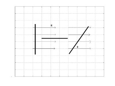 The diagram shows an electric field in the x direction with magnitude E. If the conductor is perpendicular to the E field, there is no induced voltage. If the conductor is aligned with the E field, the induced voltage is E·l where l is the length of the wire. If the angle between the E field and the wire is θ then the induced voltage is E·cos(θ)·l.
Suppose the conductor's shape is given by a curve C, and we have a vector E field E(x,y); we would like to be able to calculate the value of the induced voltage in the conductor. We can approximate the curve C with a sequence of short straight line segments of length h, such that the E field magnitude and direction are approximately constant on each segment, and then calculate the induced voltage by summing the voltages for each segment. If we reduce the size of h, this sum will approach a limit, and this limit is called the line integral of E(x,y) over C and denoted by

We will see how several line integrals are evaluated below.
If the curve C is closed (i.e. a loop), then the line integral over C is referred to as a contour integral and denoted by

A contour integral is a line integral over a closed curve.
Equation 3 - Faraday's Law of Induction
Ampere observed that a force is exerted on a moving charged particle in a static magnetic field (see Ampere's circuital law below). Thus, a force will be exerted on the electrons in a wire moving in a static magnetic field. Suppose that we have a magnetic field directed out of the screen and we have a loop of wire as shown below that is moving to the right.
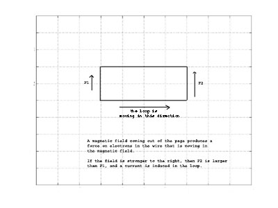 Further, assume that the strength of the magnetic field constant in the north-south direction and increases toward the right of the screen
(the east). The forces on the electrons in the top and bottom horizontal wires cancel, and since the magnetic field is stronger to the right, the force on the electrons in the right side of the loop is stronger than the force on the electrons on the left side of the loop. As a result, current will flow in the loop.
Further, assume that the strength of the magnetic field constant in the north-south direction and increases toward the right of the screen
(the east). The forces on the electrons in the top and bottom horizontal wires cancel, and since the magnetic field is stronger to the right, the force on the electrons in the right side of the loop is stronger than the force on the electrons on the left side of the loop. As a result, current will flow in the loop.
Another way of viewing the experiment above is that since the magnetic field is stronger to the right, as the loop moves to the right the magnetic flux inside the loop is increasing, and that this increase is producing the electromotive force.
It is also possible to produce a changing magnetic field in the interior of a coil without moving the coil physically. Note that if a wire is formed into a coil, and a current passed through the wire, the magnetic fields of each loop will point in the same direction and they will reinforce each other. Thus a coil of wire can be used to produce a strong magnetic field. Faraday observed that if two coils were placed in close proximity, and the current in one of the coils made to vary, it would produce a current in the other coil.
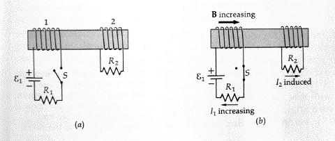 In the diagram to the left, the magnetic field produced by the coil on the left extends through the coil on the right. As the current in the left coil is varied, the strength of the magnetic field passing through the coil on the right varies, inducing a current in that coil.
The iron core pictured in the diagram has the effect of strengthening the magnetic field.
Faraday summarized the results of his experiments by the equation (Faraday's law)
EMF = dφ/dt, where
EMF is the induced electromotive force in a loop, and
dφ/dt is the rate of change of the magnetic flux passing through the loop.
Note that when Faraday performed his experiments, he could create a loop of wire, put it in a changing magnetic field, and measure the induced voltage. He could verify experimentally that the induced voltage depended only on dφ/dt, and not on the shape of the loop.
Note that at each point in the loop, the voltage is produced by the component of the E field that acts along the wire. So, if the wire is aligned with the field, the voltage produced is E*l where E is the magnitude of the field and l is the length of the wire. If the field is at right angles to the wire, then it produces no voltage. Generally, the voltage produced on a straight section of wire of lenght l is E*l*cos(α) where α is the angle beween the field direction and the wire. So, Faraday's Law of Induction can be written in integral form as
= dφ/dt
where C is any closed curve, E is the induced electric field, and dφ/dt is the rate of change of the magnetic flux inside C.
Equation 4 - Ampere's Circuital Law
The existence of the magnetic field surrounding a current carrying wire was discovered by Ampere in 1820. He discovered that two wires carrying a current exerted a force on each other. Note that even when a current is flowing in a wire, the wire is electrically neutral because the electron density in the wire is matched by the proton density. Hence, the force Ampere observed was not due to an electrical field. Ampere concluded that the force was due to magnetic fields produced by the wires, the shape of the magnetic field around a current carrying wire is shown in the diagram above.
The next question Ampere asked was "What is the strength of the magnetic field at a distance R from the wire?" The result is Ampere's Circuital Law which states
B = u0·I / (2πR) where
B is the magnetic field strength in webers / m2
u0 is the magnetic permeability of free space,
and I is the current in the wire.
Everything else follows from this equation. Note that if you have a circular loop of radius R around a wire carrying current I, the magnetic field produced by the current is aligned with the loop, so if we take the component of the magnetic field aligned with the path, and integrate it over the entire length of the path, we get
[u0·I / (2πR)] ·(2πR) = u0·I
and this value is independent of the radius of the loop.
Thus for any circle C enclosing the wire, we have
 = u0·I
We will show that the equation above holds for any (2-d, for simplicities sake) curve enclosing the wire (i.e., it doesn't have to be a circle). We'll show it by showing that it is true for curves consisting of straight line segments, and then, any curve can be approximated .... etc. Suppose we are calculating the line integral of E over the horizontal line shown in the diagram to the left.
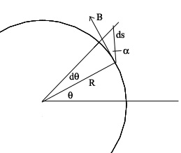 The magnitude of B at (x,y) is B1 / R where B1 is the magnitude at distance 1. As θ increases by dθ, the contribution to the line integral is given by
[B1 / R] · cos(θ) · ds, and,
R· dθ / ds = sin(90 - θ), so ds = R·dθ / cos(θ)
so that the contribution is B1 · dθ, and depends only on dθ, not the direction or location of the line!
So, we have the integral form of Ampere's Circuital Law (prior to Maxwell)
= u0·I
for any closed curve C, where I is the current enclosed by C.
In the circuit shown in the diagram the magnetic field around the parallel plate capacitor is identical to the magnetic field around the wire. However, if the plane of the loop C passes between the plates of the capacitor, the current enclosed by the loop is 0 and Ampere's law as written above will not give the correct result.
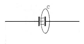 Maxwell hypothesized that the changing electric flux between the plates of the capacitor creates a magnetic field. He added a term to Ampere's Circuital Law to account for this, giving
= u0·I + u0·dφ/dt
Maxwell hypothesized that the changing electric flux between the plates of the capacitor creates a magnetic field. He added a term to Ampere's Circuital Law to account for this, giving
= u0·I + u0·dφ/dt
for any closed curve C, where I is the current enclosed by C and φ is the electric flux enclosed by C. Note: for a parallel plate capacitor, φ=e0E·A where E is the electric field between the plates and A is the plate area.
The Differential Form of Faraday's Law of Induction
Maxwell's equations can be written in integral and differential form. Now, we want to derive the differential forms of the last two equations, with the goal of getting to the wave equation for electromagnetic radiation.
We want to be able to write Faraday's Law as a differential equation, so we will examine what it says about the electrical and magnetic fields in the close vicinity of a point in a changing magnetic field. Faraday's Law says that a changing magnetic field will produce a current in a loop, that is, it will create a force on electrons in a wire, and we will represent this force by an electric field E(x,y) = (Ex(x,y), Ey(x,y)), where we have reduced the spatial dimensions to two for simplicity.
Suppose that the magnetic field B is directed out of the screen, and its magnitude is given by B(x,y,t), and that we have a small wire loop located at the point (x,y) as shown in the diagram. Consider the electromotive force in the loop created by the x component of the electric field E at the instant t.
 The x component of E does not create any emf acting on the left and right vertical sides of the loop. The voltage created in the lower horizontal wire is (approxmately)
Ex(x, y)·h
and the voltage created in the upper horizontal wire is
Ex(x, y+k)·h
Similarly, the voltage created in the left vertical wire is given by
Ey(x, y)·k
and the voltage created in the upper horizontal wire is
Ey(x+h, y)·k
So, the total induced voltage in the loop, with the clockwise direction being positive, is
[Ex(x, y+k)·h - Ex(x, y)·h] - [Ey(x+h, y)·k - Ey(x, y)·k]
That is, = [Ex(x, y+k)·h - Ex(x, y)·h] - [Ey(x+h, y)·k - Ey(x, y)·k]
From Faraday's Law of Induction we know that this voltage equals dφ/dt where φ is the total magnetic flux in the loop. But, φ approximately equals the value of the magnetic field at (x, y) times the area of the loop, that is, h·k, so, we have
[Ex(x, y+k)·h - Ex(x, y)·h] - [Ey(x+h, y)·k - Ey(x, y)·k] = dB(x,y,t)/dt·h·k
Divide both sides of the equation by h·k, then let h and k approach zero, giving
 -
-  = dB/dt
In words, if the x component of E is increasing with y, then the induced voltage in the top horizontal wire is stronger than that in the lower horizontal wire, so there is a net positive voltage around the loop.
If the y component of E is increasing with x, then the induced voltage in the left vertical wire is less than the induced voltage in the right vertical wire, and hence there is a net voltage drop around the loop.
As the loop becomes smaller, the induced voltage in the loop divided by the area of the loop approximates the rate of change of the magnetic field.
The Differential Form of Ampere's Law
We can use a diagram just like the one above, but we'll assume (the reason will be clear below) that the current is in the y direction (and hence the diagram to the left represents the x and z axes).
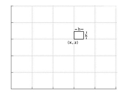 From the integral form of Ampere's circuital law we have that the line integral around the small loop equals the current through the loop. The line integral can be evaluated just as we did above for E, giving
= [Bx(x, z+k)·h - Bx(x, z)·h] - [Bz(x+h, z)·k - Bz(x, z)·k]
So, from Ampere's Circuital Law we have
[Bx(x, z+k)·h - Bx(x, z)·h] - [Bz(x+h, z)·k - Bz(x, z)·k] =
u0·ρ·h·k + u0e0·dE/dt·h·k
where ρ is the current density and e0E is the electric flux density. Dividing by h · k and letting h and k go to 0 gives
 -
-  = u0ρ+ u0e0dE/dt
Derivation of The Wave Equation for Electromagnetic Radiation
We have Faraday's Law of Induction,
- = dB/dt
and, in free space there are no currents, so Ampere's Circuital Law becomes
- = u0e0dE/dt
We will assume that the magnetic field is everywhere pointing in the z direction. As it changes, by Faraday's Law of induction, it produces an electric field in the x-y plane, and we will assume that it is everywhere in the y direction. With these assumptions, can we come with a solution to the two DEs above?
Since Ex = Ez == 0, we can write Faraday's Law of Induction, with Ey = E and Bz = B, as
 = -
= - 
That is, a spatial E field 'differential' produces a changing B field.
Ampere's Circuital Law becomes
 = - (1/e0u0)
That is, a spatial B field 'differential' produces a changing E field.
Taking the second partial derivative of E wrt time gives
 = - (1/e0u0)
Taking the spatial derivative of Faraday's Law gives
 = -
= - 
Noting that = and substituting gives the wave equation for electromagnetic radiation
= (1/e0u0)
Light is Electromagnetic Radiation
Fairly accurate estimates of the speed of light, obtained by timing celestial events, date from before the time of Newton. The wave equation also gives a speed for the propagation of electromagnetic radiation, that is 1 / sqrt(e0u0). Maxwell noticed that these were in agreement. Until that time no one knew what light was.
Further consideration of the speed of light, and a pivotal experiment, motivated the development of the special theory of relativity a few years later.