Calculus Without Tears
An Airplane Simulator
Introduction
An airplane simulation illustrates how differential equations, and Newton's Second Law of motion, both familiar to readers of CWT, are used to study motion. And, it gives us an opportunity to use multi-variable functions, and vectors, to analyze familiar phenomena. The primary technique of the simulation is the method of computing numerical solutions to differential equations covered in CWT Vol. 2 Chapter 2, i.e. we use our favorite formula distance = velocity * time.
Vectors
A vector is a directed line segment, like an arrow. It has a length, also called its magnitude, and a direction. Below we will simulate an airplane flying in two-dimensional space (three is more complicated), and we will use two-dimensional vectors to represent the airplane's velocity, the thrust of the airplane's engine, lift, and drag. We will specify a vector by specifying its two components, that is its component in the horizontal (x) direction, and its component in the vertical (y) direction. For example the velocity vector with x component 5 and y component 0 represents a velocity of magnitude 5 in the x direction. A velocity vector with x component 0 and y component 5 represents a velocity of magnitude 5 in the y direction. A velocity vector with x component 6 and y component 6 represents a velocity of magnitude (62+ 62)1/2 = 8.5 and direction π/4 radians as shown in the diagram. The direction of a vector is specified by the angle it makes with the x axis.
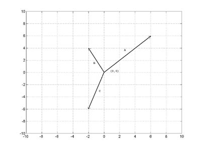 The components of the vectors in the diagram are
a - (6, 6)
b - (-2, 4)
c - (-2, -6)
The Airplane
The airplane control surfaces are shown in the diagram below.
 We will simulate the effect of only one of these control surfaces, the elevators on the tail of the airplane. When the pilot pulls back on the joystick or steering yoke of the plane, the elevators tilt up, causing a downward force on the tail of the plane which causes the nose to pitch up.
If the pilot pushes the joystick or steering yoke forward, the elevators tilt down causing an upward force on the tail which causes the the nose of the plane to pitch down.
The Motion of a Rigid Object
Think of a baseball thrown by a pitcher: as it travels toward the catcher, the ball 'as a whole' is moving in a more or less straight line, but, the ball is also spinning, so that at any instant the different points in the ball are travelling at different speeds and different directions! Fortunately, it is possible to decompose the motion of a rigid body into two parts, the motion of one point, the center of mass, and the rotation of the object about its center of mass. Thus, we can accurately describe the motion of the ball by specifying at each instant the location of the center of mass and the rotation of the ball about its center of mass.
To specify a rotation in 3-dimensional space it is necessary to specify an axis of rotation as well as the amount of rotation. The axis of rotation can change from moment to moment, and it is a tricky business to keep track of it. However, if we restrict the motion of our airplane to two dimensions, x (forward/backward) and y (up/down), then the axis of rotation will be fixed (the z or pitch axis), and we can specify the motion of the plane by specifying the motion of the center of mass and the rotation about the center of mass expressed as an angle.
If a force acts on a rigid body, and the direction of the force is along the line throught the point of application thru the object's center of mass, then it will cause the
 object to accelerate according to Newton's Second Law of Motion, and that's it. However, if the force is not directed through the center of mass it will also cause the object to rotate. Suppose the center of mass of the object shown to the left is at point p, and a force f is applied to the object. This force will cause the entire object, including point p, to accelerate according to Newton's Second Law of Motion. The force f also produces a torque at point p and an angular acceleration about p according to Newton's Second Law for rotation, which is
α'' = T / I
where α'' is angular acceleration, I is the object's moment of inertia about its center of mass, and T is the applied torque. If there are no other forces acting on the object it will tumble, as shown below.
An object's moment of inertia depends on how the object's mass is distributed about the center of mass. We will assume that the plane's center of mass is located 1/3 of the way back from the nose, and that the plane's moment of inertia about this point is given by 1/20 * m*L2 where m is the mass of the airplane and L is the plane's length (for a discussion of moments of inertia see Common Moments of Inertia)
Airplane Dynamics, Abbreviated, Part 1, the Differential Equations
The trajectory of the airplane is a solution to the DE given by Newton's Second Law of Motion, that is, F = m*A. If p(t) = (px(t), py(t)) is the trajectory of the airplane's center of mass, then px(t) satisfies the DE
px''(t) = Fx(t) / m
and py(t) satisfies the DE
py''(t) = Fy(t) / m
where F(t) = (Fx(t), Fy(t)) is the sum of the forces acting on the airplane at time t.
If α(t) is the pitch angle of the airplane, then α(t) satisfies the DE given by Newton's Second Law for rotation, that is,
α(t)''(t) = T(t) / I
where T(t) is the sum of the torques acting on the airplane's center of mass at time t and I is the airplane's moment of inertia about its center of mass.
So, if we know the airplane's initial position, velocity, pitch, and pitch rate, and we are able to calculate F(t) and T(t) as time progresses, then we can subdivide time into small subintervals of length h, calculate px''(0), py''(0), and α''(0), use these values to calculate px'(h), py'(h), and α'(h), then use these values to calculate px(h), py(h), and α(h). and we're on our way to calculating a solution to the DEs above, that is, the airplane's trajectory. We repeat this process to generate a numerical solution through time. This is exactly the same thing that we did in CWT Vol. 2 Chapter 2. Remember that the calculations in CWT Vol. 2 Chapter 2 are based on our favorite formula distance = velocity * time, and its more general form, change = rate of change * time.
An Interlude, Simulating a Rigid Body Tumbling in Space
Let's stop right here and simulate the motion of our plane as it moves through space acted on only by the force of a small thruster located on the plane's tail and pointing downward. We'll assume that we're in outer space so that there is no gravity, drag or lift (to make it easy).
Initialize constants and the initial state
x = 0; % initial x position of airplane center of mass
y = 0; % initial y position of airplane center of mass
pa = 0; % initial pitch angle
vx = 35; % initial x velocity
vy = 35; % initial y velocity
vpa = 0; % initial pitch angle rate
m = 1; % airplane mass (it's a model plane)
L = 1; % airplane length
I = 1000; % airplane moment of inertia (chosen to give interesting graph)
thrust = -1; % force of thruster in newtons
dt = 1; % time increment
The loop advances time, where time = i*dt
for i = 1:300
The thruster angle is the pitch angle plus 90 degrees (pi/2 radians)
ta = pa + pi/2; % thrust angle at ti-1 is plane angle plus 90 degrees
xthrust = -thrust * cos(ta); % compute thrust in x direction at ti-1
ythrust = thrust * sin(ta); % compute thrust in y direction at ti-1
xaccel = xthrust / m; % compute x acceleration at ti-1, a=F/m
yaccel = ythrust / m; % compute y acceleration at ti-1, a=F/m
x = x + vx*dt + xaccel*dt*dt/2; % compute x position at time ti, d=v*t plus square correction term
y = y + vy*dt + yaccel*dt*dt/2; % compute y position at time ti, d=v*t
vx = vx + xaccel*dt; % compute x velocity at time ti, change in v = a*t
vy = vy + yaccel*dt; % compute y velocity at time ti, change in v = a*t
The distance from the thruster to the center of mass is 2*L/3, and the torque equals the thruster force times that distance
paaccel = -thrust * (2*L/3) / I; % compute angular acceleration Newton's 2nd law for rotation
pa = pa + vpa*dt + paaccel*dt*dt/2; % compute pa at time ti, d=v*t
vpa = vpa + paaccel*dt; % compute vpa at time ti, change in angle velocity = angle accel*t
px(i) = x; % save the trajectory values so we can graph them later
py(i) = y;
angle(i) = pa;
end
A graph of the object's trajectory, that is, p(t) = (px(t), py(t)) plotted as a function of time, would require a 3-dimensional graph, which is more than we want to attempt right now. So, instead we will plot py(t) on the y axis and px(t) on the x axis. This graph shows the where the object went as time progressed, but it does not show speed.
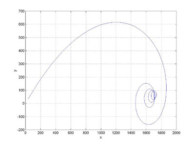
plot(px(1:300), py(1:300))
We can also plot the object's pitch angle as a function of time, this graph shows that the object rotated (30 / 2*pi) = 4.77 times.
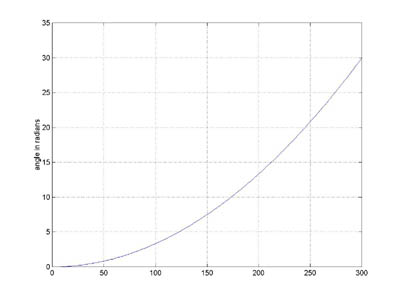
plot(angle(1:300))
Aircraft Dynamics, Abbreviated, Part 2, Calculating Forces and Torques
Now it's time for the hard work, so, we may cheat a little. The forces acting on an airplane in flight are shown in the diagram below.
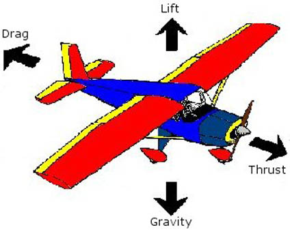 In addition to the forces shown, we will also model the effect of elevator activation, that is, a force applied at the tail of the airplane resulting in a torque about the plane's pitch axis.
For simplicities sake, our plane will be two-dimensional and fly in two-dimensional space. Thus, our plane looks like the diagram below:
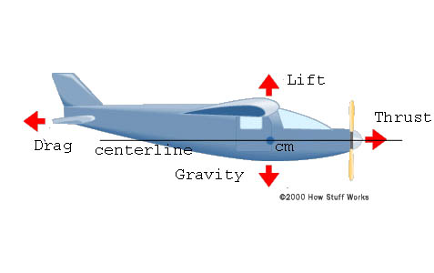 The x coordinate will represent the aircraft's horizontal position and the y coordinate the aircraft's altitude. We'll describe the aircraft's trajectory and attitude by specifying for each instant in time the x and y coordinates of the aircraft's center of mass (cm), and the aircraft's pitch angle, that is, the angle between the aircraft's centerline and the x axis.
The 'state' of the aircraft at a particular instant will consist of the aircraft's
- position
- velocity
- pitch angle
- the angular rate of the pitch angle
At each point in time we'll need to be able to calculate the forces acting on the airplane. We will have the airplane's state information available to us to use in these calculations.
The Forces and Torques Acting on the Airplane
Each force acting on the airplane is represented by a vector, and we'll have to calculate the the magnitude and direction of these vectors.
Gravity -
We'll assume constant gravity acting straight down. Hey, this one was easy.
Thrust -
Thrust is produced by the plane's engine and controlled by the throttle. We'll assume that thrust magnitude is constant and directed along the centerline of the aircraft. Can they all be this easy?
Lift and Drag -
Things get considerably more complicated here. Both lift and drag are created by the air as the airplane travels through it. Surprising to me, the phenomena of lift is still controversial, see, for example, Airfoil Lifting Force Misconceptions. Generally, lift and drag can be modeled by equations of the form
Lift = (1/2) · d · v2 · s · CL, where
d is the density of air
v is magnitude of the airplane's velocity
s is the lifting surface area
and CL is the lift coefficient, which is critically dependent on the airplane's angle of attack.
Note that the centerline of the airplane does not necessarily line up with the airplane's velocity vector. The angle between these vectors is called the airplane's angle of attack.
 Typically an airplane flies with a small, non-zero, angle of attack. When the pilot pulls back on the joystick or steering yoke, the tail goes down and hence the angle of attack increases, increasing lift, and the plane goes up.
The diagram to the left shows the relationship between CL and angle of attack for a typical airplane.
We have all the information available to use the above model, but, we don't want to go there. So, we'll use an easier model, that is, we'll assume just enough lift to cancel gravity, and assume a constant drag. This is a cop out, but, complicated flight dynamics are not our focus here.
Elevator Torque -
When an elevator is moved into the airstream, it generates a up/down force applied at the tail of the plane (as well as a small amount of drag that we will ignore).
We will assume that all the forces (except that caused by the elevator) are directed through the planes center of mass and do not create any torques on the plane.
The program will vary the elevator torque to simulate pilot control.
Let's Fly
We 'fly' the simulator by running the program. The only control is the elevator which is programmed below.
Initialize constants, the initial state, etc.
x = 0; % initial x position of airplane center of mass
y = 1000; % initial y position of airplane center of mass
pa = 0; % initial pitch angle
vx = 15; % initial x velocity in m/sec second
vy = 0; % initial y velocity
vpa = 0; % initial pitch angle velocity
m = 2; % airplane mass is 2 kg (it's a model plane)
L = 1; % airplane length is 1 m
I = (1/20)*m*L*L; % airplane moment of inertia about cm
D = (1 / 15); % drag coefficient converts 30 km/hour to 1 newton drag
tprop = 1; % 1 newton, should maintain level flight at 30 km/sec
dt = 1; % time increment
The loop advances time, where time = i*dt
for i = 1:300
The propeller thrust is along the centerline of the aircraft, resolve it into x and y components
fxprop = tprop * cos(pa); % compute propeller thrust in x direction at ti-1
fyprop = tprop * sin(pa); % compute propeller thrust in y direction at ti-1
vmag = sqrt(vx*vx + vy*vy); % magnitude of the velocity at ti-1
fxdrag = - D * vx;
fydrag = - D * vy;
We perform detailed calculations of lift (omitted), and notice that it is exactly canceled by gravity. Fortunate!
xaccel = (fxprop + fxdrag) / m; % compute x acceleration at ti-1, A=F/M
yaccel = (fyprop + fydrag ) / m; % compute y acceleration at ti-1, A=F/M
x = x + vx*dt + xaccel*dt*dt/2; % compute x position at time ti, d=v*t
y = y + vy*dt + yaccel*dt*dt/2; % compute y position at time ti, d=v*t
vx = vx + xaccel*dt; % compute x velocity at time ti, change in v = a*t
vy = vy + yaccel*dt; % compute y velocity at time ti, change in v = a*t
Here we assign values for the elevator force, this is more or less arbitrary
if (i < 50)
ef = 0; % fly level for a while
elseif (i < 150)
ef = 0.00001; % then tail down, nose up, plane goes up
else
ef = -0.00003; % then tail up, nose down, plane descends
end
Compute the rotation dynamics
paaccel = ef * (2*L / 3) / I; % compute angular acceleration Newton's 2nd law for rotation
pa = pa + vpa*dt + paaccel*dt*dt/2; % compute pa at time ti, d=v*t
vpa = vpa + paaccel*dt; % compute angular velocity at time ti, change in angle velocity = angle accel*t
px(i) = x; % save the trajectory values so we can graph them later
py(i) = y;
angle(i) = pa;
end
py(t) is plotted on the y axis and px(t) on the x axis in the graph below:
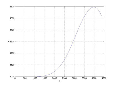
plot(px(1:300), py(1:300))
Hey, what did you expect, a party with special hats and noisemakers ?
Well ... why not .....