
Calculus Without Tears
Synopsis of Mathematical Modeling and Computational Calculus I
Introduction
This book will take you from not being able to spell ‘calculus’ to doing calculus just the way I did it for twenty years as an engineer at high tech firms like Lockheed and Stanford Telecom. You will learn how physical processes are modeled using mathematics and analyzed using computational calculus. Systems studied include satellite orbits, the orbits of the earth and moon, rocket trajectories, the Apollo mission trajectory, the Juno space probe, electrical circuits, oscillators, filters, tennis serves, springs, friction, automobile suspension systems, lift and drag, airplane dynamics, and robot control. And not a single theorem in sight.
This book focuses on differential equation models because they are what scientists and engineers use to model processes involving change. Historically, this has presented a problem for science education because while creating a model is usually straightforward, solving the model differential equations is usually impossible, that is, most differential equations do not have analytic solutions. This has been a tremendous roadblock to science and science education. But, that was before computers; now, with computers, solutions to differential equations can be computed directly, without the need for an analytic solution, and without advanced mathematics, using the formula distance equals velocity times time. It’s just that simple. The book will show you how it’s done.
Constant Velocity Motion
We start from ground zero and cover calculus as applies to constant velocity motion. Everything there is to know about constant velocity motion is in the formula distance = velocity * time, so there are no mysteries here.
Constant velocity motion is represented mathematically by a function of form p(t) = V*t + P0 where V is the velocity and P0 is the starting point, i.e. the position at time t = 0. Note: we italicize function names, p is for position.
The derivative of a function is the rate of change of the function, the derivative of p(t) is denoted by p'(t). If p(t) represents constant velocity motion with velocity p(t), i.e. p(t) = V*t + P0, then the velocity of the motion is V for every value of t and so p'(t) = V.
Suppose we have a position function p(t) but that we do not know the equation defining it. The function is unknown ! But, suppose we do know that the velocity of the motion it represents is constant and equals 5, then we can write a differential equation
p'(t) = 5
where we've written the function name in bold letters to remind us that its definition is unknown. An equation containing the derivative of an unknown function is called a differential equation. To solve this differential equation we need to find a definition of p(t) that makes the differential equation true. Can you solve this differential equation? Hint: see the previous paragraph.
Mathematical Model of a Falling Object
According to the story he told himself, Newton discovered the Law of Universal Gravity after watching an apple fall from a tree on his country estate. Gravity is the force that pulls the apple toward the earth and causes it to fall. It also acts on the moon to hold it in its orbit. The formula, it could have been a lucky guess, is:
F = G * Mearth * Mapple / (R * R), where
G is the gravitational constant
Mearth is the mass of the earth
Mapple is the mass of the apple
R is the distance between the centers of earth and apple
Having discovered gravity, Newton understood that there was a force acting on the apple; now he wanted to understand the apple’s trajectory as it falls, that is, he wanted to know the position function for a falling apple. First, he needed to know how the force of gravity affects the apple's trajectory, and to this end he discovered the Second Law of Motion (after discovering the First Law of Motion), which is force (F) equals mass (M) times acceleration (A), or
F = M * A.
Putting the two formulas together gives us Newton's model for a falling apple, that is,
G * Mearth * Mapple / R2 = Mapple*A
Note that Mapple divides out of the formula, giving
A = G * Mearth / R2
Graphing Solutions to Differential Equations
If the apple is close to the surface of the earth then R ~ the radius of the earth for the entire trajectory, and substituting the numbers in the formula above gives
A = 9.80665 ~ (-)10 m/sec2
This is a constant acceleration model and is a simplified model for a falling object taught in high school and introductory university physic courses. We know that the solution to the differential equation v'(t) = -10 is v(t) = -10 * t + V0. That is, if we drop the ball at time t = 0 with initial velocity 0, then after 1 second its velocity is -10 m/sec, after 2 seconds its velocity is -20 m/sec, and so on.
How can we plot the trajectory of a falling apple, using our simple model p’(t) = -10 * t + V0, with V0 = 0 ? As the apple falls its downward velocity increases, so we're not dealing with our favorite type of motion, constant velocity motion. Can we convert the problem into a constant velocity problem? We can. Suppose we want to compute the trajectory for 10 seconds, what we can do is divide the time interval into shorter subintervals, and assume that the velocity is constant on each subinterval ! This is how we do it.
We start by dividing the 10 second interval into two 5 second subintervals. We need a velocity for the 1st subinterval, and we'll choose the apple's velocity at the start of the subinterval.
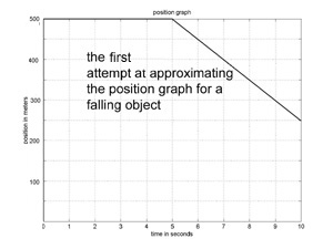 Since we are starting our trajectory just when the apple starts falling, its initial velocity is 0. So, our approximate trajectory will have velocity 0 for the first 5 seconds. A graph of the approximate trajectory is shown to the left, and it is a horizontal line for the first 5 seconds. Not such a great start. How about the velocity for the 2nd subinterval? The apple's velocity at the start of the 2nd subinterval is p’(5) = -10 * 5 = -50, so that is the velocity we use for the second subinterval. So, we have the approximation to the trajectory of a falling apple shown. Not so great, but, we're just getting started.
The problem with our first approximation is that the subinterval size was too large. If we divide the 10 seconds into 10 one second intervals, and follow the method used above to produce a linear approximation for each subinterval, we get the graph to the left. This is a pretty 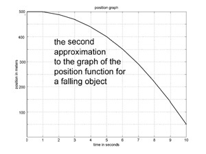 good approximation to the true trajectory of a falling apple.
Computing Approximate Solutions to Differential Equations Using Euler's Method
A system model consists of a set of state variables that determine the state of the system, and a rate (i.e. differential) equation that calculates the rate of change for each state variable. Newton's model for a falling apple has two state variables, the apple's position (distance from the center of the earth) r and the apples velocity v. The rate equations are
r’(t) = v(t)
v’(t) = - G * Mearth / r(t)2
The computational equations for calculating an approximate trajectory for a falling apple using Newton's model are, with r(t) = p(t) + rEarth,
p(t+dt) = p(t) + p'(t)*dt = p(t) + v(t)*dt
v(t+dt) = v(t) + v'(t)*dt = v(t) - (G * Mearth / r(t)2)*dt
To calculate an approximate trajectory the time interval of interest, say 10 seconds, is divided into short subintervals, and the computational equations are used to project the solution over each subinterval.
Here we calculate an approximate trajectory for by dividing a 10 second interval into five 2 second subintervals
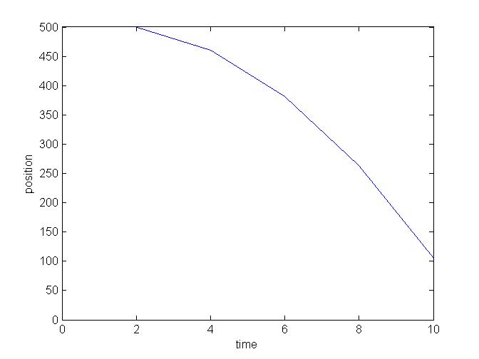
p(0) = 500 and v(0) = 0
p(2) = p(0) + v(0) * 2 = 500 + 0 * 2 = 500
v(2) = v(0) + (- G * Mearth / r(0)2) * 2 = 0 + 0 * 2 = 0 - 9.8*2 = -19.7
p(4) = p(2) + v(2) * 2 = 500 + 0 * 2 = 500 + (-19.7)*2 = 460.5
v(4) = v(2) + (- G * Mearth / r(2)2) * 2 = -19.7 -9.8 * 2 = -19.7 - 9.8*2 = -39.1
p(6) = p(4) + v(4) * 2 = 460.5 + 0 * 2 = 460.5 + (-39.8)*2 = 381.7
v(6) = v(4) + (- G * Mearth / r(4)2) * 2 = -39.8 -9.8 * 2 = -39.1 - 9.8*2 = -58.8
etc.
The computational equations above translate directly to MATLAB statements. MATLAB is the industry standard programming language for engineering applications; the basic language hasn’t changed in thirty years, and only the basic features are used, plus the graphing functions. Each program consists of three sections, 1 - the initialization of constants and variables, 2- the loop that advances the solution thru time, 3 – graphing the results. See the program for Newton's model here
An Ounce of Trigonometry
We will be modeling 2-dimensional processes, e.g. orbits (a falling object in 2-d), and that requires a little bit of trigonometry to resolve vectors into their x and y components, essentially the trig necessary to convert from rectangular to polar coordinates and back, that is (x, y) = (R, a)p where R = (x2 + y2)1/2 and a = sin-1(y/R), and (R, a)p = (R*cos(a), R*sin(a)), and that's it, folks.
Introduction to MATLAB/OCTAVE/FREEMAT
. MATLAB is the industry standard programming language for engineering applications; the basic language hasn’t changed in thirty years, and only the basic features are used, that is, assignement statements, for loops, and an occasional if statement, plus the graphing functions. Each program consists of three sections, 1 - the initialization of constants and variables, 2- the loop that advances the solution thru time, 3 – graphing the results.
The downside of MATLAB is that it is not free. Fortunately two completely free and legal clones are available, FREEMAT and OCTAVE. The clones execute exactly the same commands as MATLAB and are for our purposes equivalent
Orbits, Satellites, Rockets
The moon, and satellites around the earth, are falling bodies and hence the mathematical model for their trajectories is the same as the model for a falling apple, with one difference, that is the
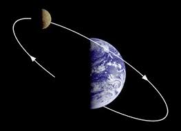 simplified model won't work, it takes Newton's model to get accurate elliptical orbits.
Using that model with the proper initial conditions produces the graph of the moon's orbit shown here: Note: the illustration is not to scale, the graph is.
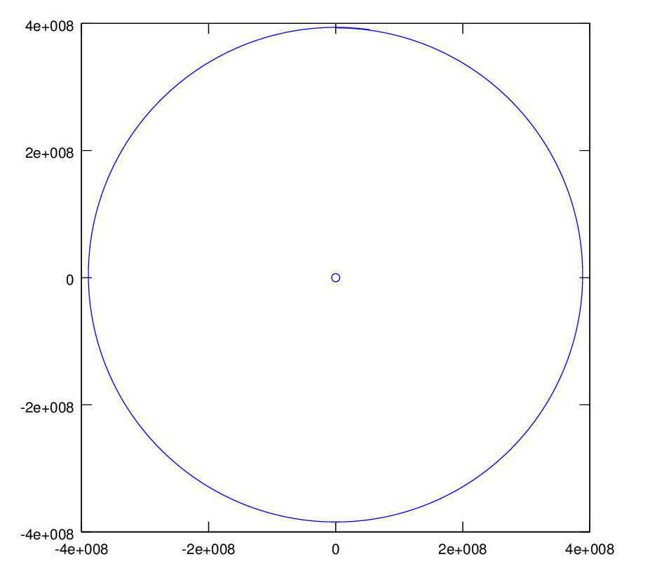
See the orbit program here
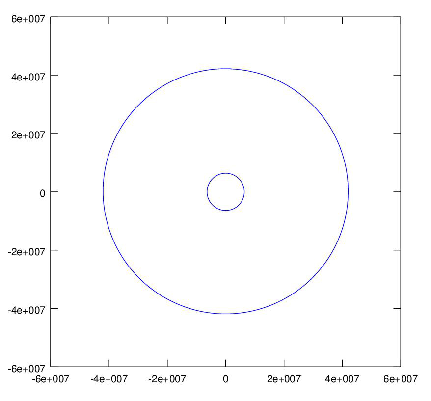
A geostationary satellite orbit has a period of 24 hours so that the satellite in orbit above the equator rotates at the same rate as the earth and appears fixed in the sky when viewed from the earth.
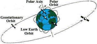
By changing the satellite initial state in the orbit program, i.e. position and velocity, we get a geosynchronous orbit, and elliptical orbit, and a hyperbolic trajectory, as shown.
&;
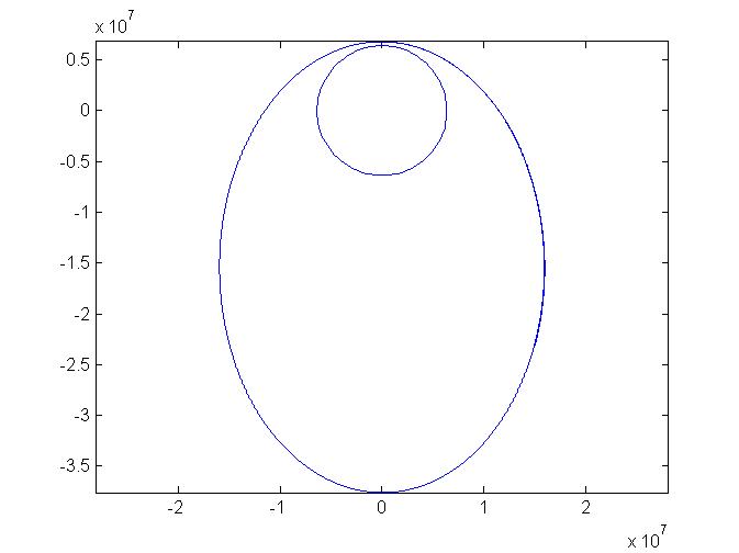
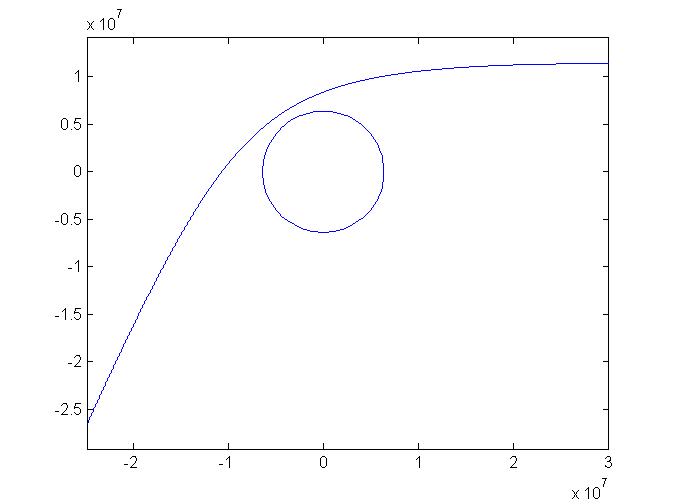
Adding a rocket to the model of the moon's orbit, we can launch (in this case shoot) the rocket straight up from the earth and adjust the initial state of the moon so that they get to the same place at the same time. A hit ! This time the moon's outline at the end of the simlation is also graphed.
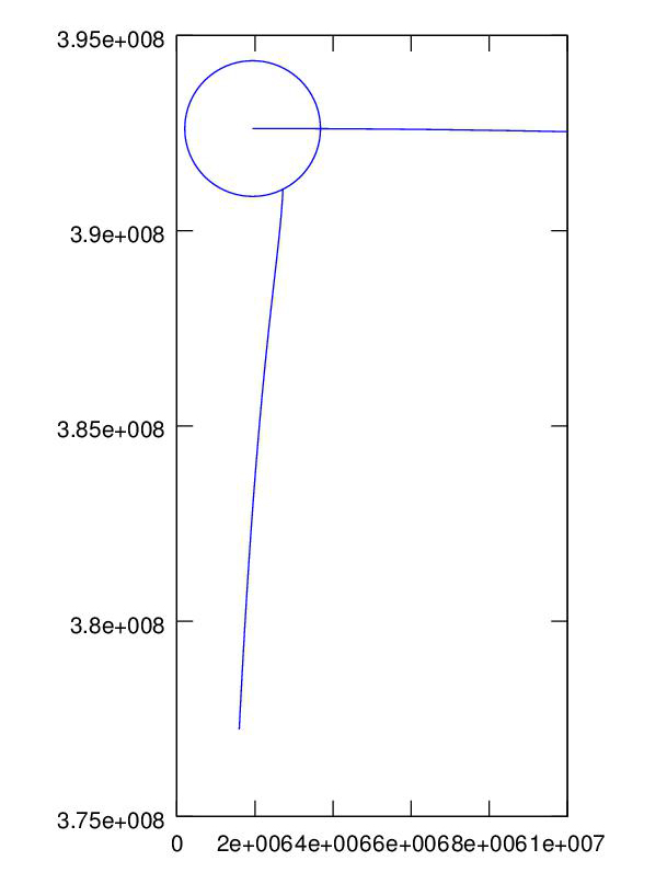
The Apollo mission did not hit the moon but rather just missed, and the lunar module went into orbit around the moon. We hit the moon in the last project, we can also miss, but no matter how closely we come to the moon, we can't get into orbit around the moon without a guidance boost, so we program a directed boost just as the rocket passes the moon, et viola'.
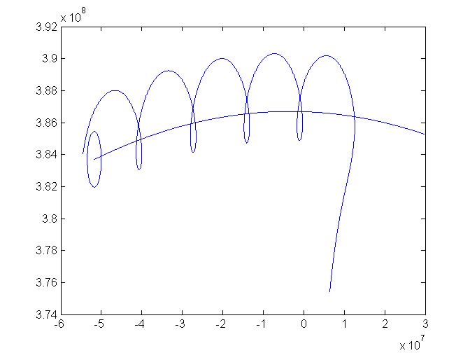 The plot shows the Apollo spacecraft going into orbit around the moon and making several orbits, the outline of the moon is drawn at its position at the end of the program run. See the Apollo program here
The US launched a probe to Jupiter on Aug. 5, 2011. The trip to Jupiter will take five years, and utilizes a
slingshot, or gravity assist, trajectory. The boost rocket put a Centaur upper stage and the Jupiter probe into a low 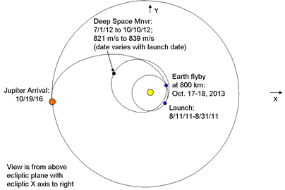 orbit around the earth. The Centaur then launched the probe into a deep space orbit around the sun that will return to the earth in two years! The gravitational field of the earth will then accelerate the probe and send it on its way to Jupiter. The flight of the probe is un-powered except for two deep space maneuvers a year into the flight. A diagram of the actual planned trajectory is shown in the figure.
It’s helpful to see an animation to understand how the slingshot works, and that can be seen here
http://www.youtube.com/watch?v=sYp5p2oL51g
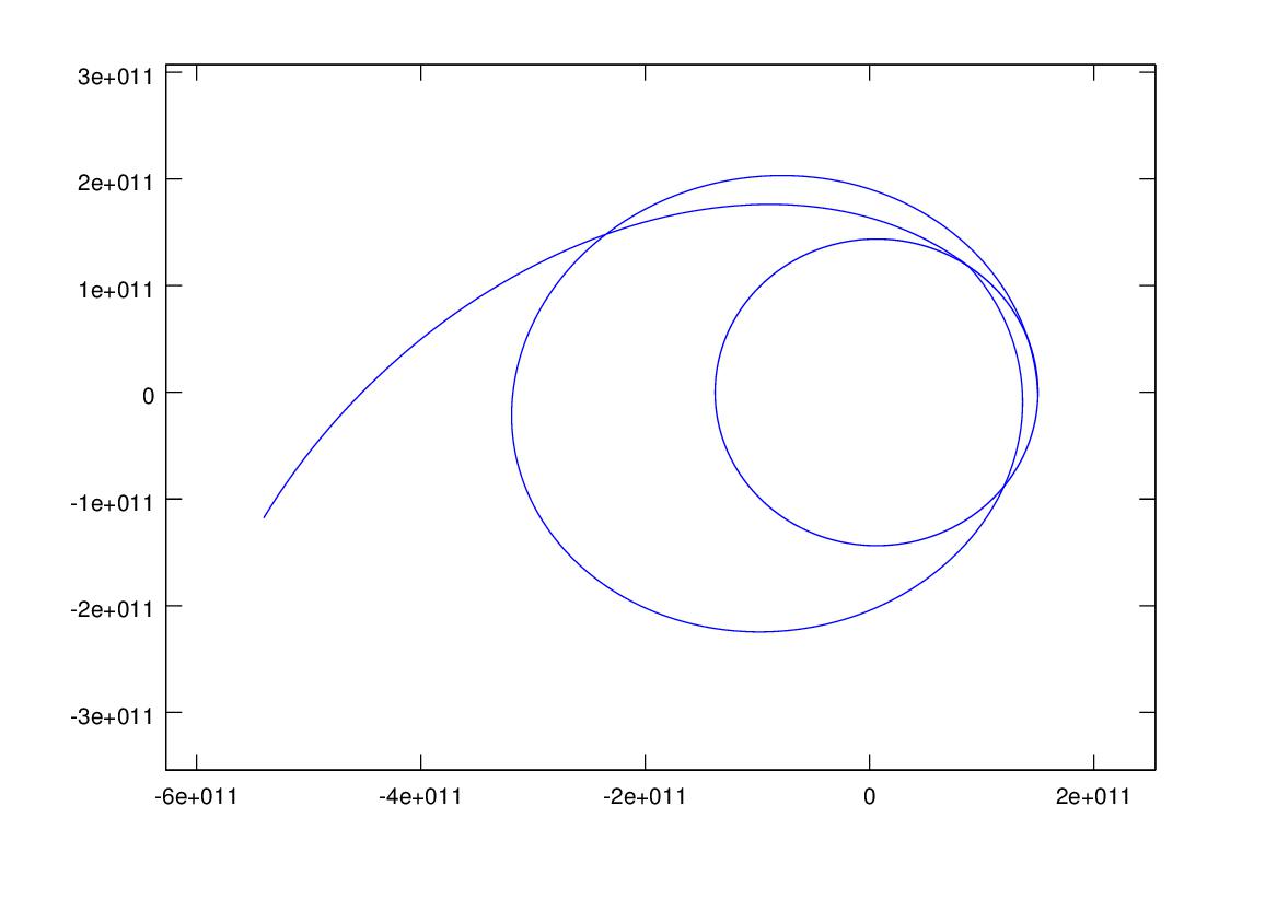
Once the probe detaches from the Centaur booster it is acted on only by the gravitational fields of the earth and the sun (minus the deep space maneuvers). The model is the falling object model times three, the earth is falling towards the sun, the rocket is falling towards the sun, and the rocket is also falling towards the earth. We program these three models and add a programmed deep space guidance boost to get the right trajectory, and viola'. The graph shows the 3 year trajectories of the earth around the sun, which traces out a circle 3 times, and the rocket, the big ellipse followed by the slingshot trajectory to the outer planets.
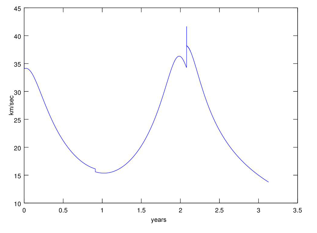
This graph shows the rocket's velocity for the entire flight, note the spike when the slingshot shoots the rocket toward Jupiter.
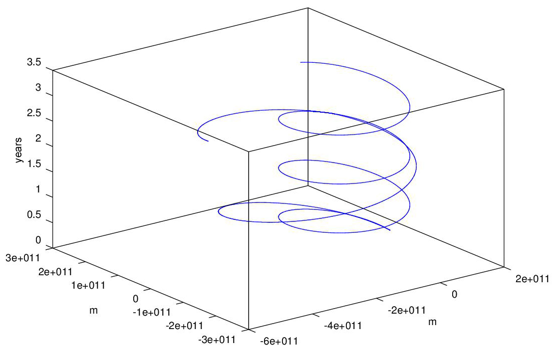
This is a 3-d version of of the graph showing the rocket and earth trajectories, plotted using the MATLAB/OCTAVE/FREEMAT plot3 command, nothing to it.
You can follow the progress of the real Juno mission here
The Rosetta mission to send a rocket to Comet 67P/Churyumov-Gerasimenko utilizes four slingshot assists, the trajectory can be seen
here.
Charley Kolhase was the mission planner for the Voyager and Cassins missions to the outer planets, working for the Jet Propulsion Laboratory. He has a series of four hour long lectures on the internet explaining how missions to the planets are planned in detail, at
here.
Electrical Circuits
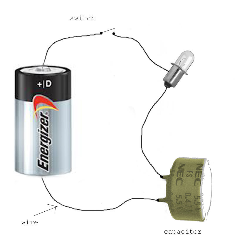
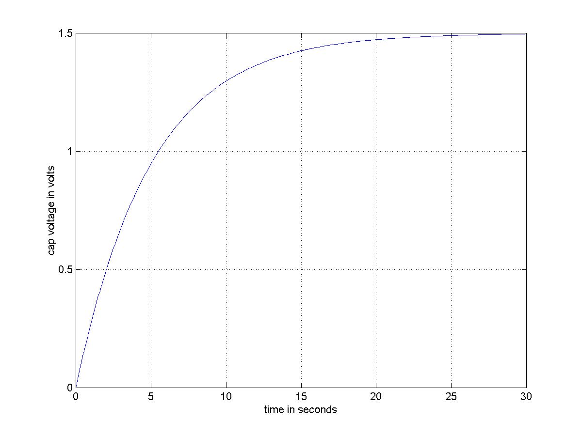
The models for the primary circuit elements are vR(t) = i(t)*R for a resistor of resistance R where vR(t) is the voltage across the resistor and i(t) is the current through the resistor, vC'(t) = i(t)/C the model for a capacitor of capacitance C, and vL(t) = i'(t)*L the model for an inductor of inductance L. The models are intuitively clear and explained fully in the book. Given a simple circuit with a battery, a resistor (the filament of a bulb), and a capacitor, Kirchoff's voltage law states that the sum of the voltages around a circuit loop is 0, so
VB - i(t)*R - vC(t) = 0
so
i(t) = (VB - vC(t))/R
and we have our differential equation model for the capacitor voltage
vC'(t) = i(t)/C = (VB - vC(t))/(R*C)
We can use graph the capacitor voltage when the switch closes as shown
An RLC oscillator circuit is shown, it includes a voltage generator VS. Our model will use two state variables, the circuit current and the capacitor voltage. From Kirchoff's voltage law VS(t) - vR(t) - vL(t) - vC(t) = VS - i(t)*R - i'(t)*L - vC(t) = 0
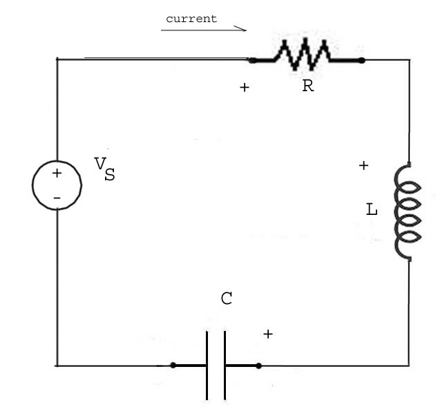
and we have a differential equation for i(t),
i'(t) = (VS(t) - i(t)*R - vC(t))/L
and the capacitor model gives us the differential equation for vC(t),
vC'(t) = i(t)/C
The computational equations are
i(t+dt) = i(t) + (VS(t) - i(t)*R - vC(t))/L*dt
vC(t+dt) = vC(t) - i(t)/C*dt
We can 'program' the voltage source by first initializing it to zero VS = zeros(1,N), and then setting non-zero values as we like. Suppose the subinterval length is 0.01 seconds and we want a unit 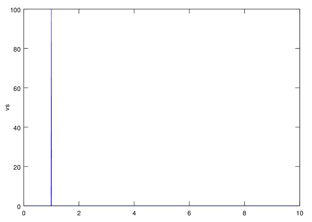 (integral) impulse to occur at 1 second into the simulation, then VS(100) = 100 does it. The graph shows the VS voltage.
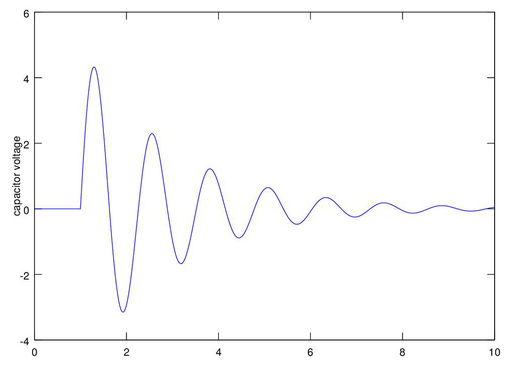
This graph shows the response of the system to a unit impulse at 1 second, see the program here.
The process of using computational calculus to analyze electric circuits has been automated, the industry standard program for circuit analysis is SPICE (Simulation Program with Integrated Circuit Emphasis). Electrical engineers routinely use SPICE to analyze newly designed circuits, see SPICE homepage and LTSPICE for pc and mac.
2-D Rigid Body Dynamics
An actual 3-d object not only moves from place to place, it rotates, think of a kick serve in tennis, the ball spins as it travels through air. The motion of a an object can be decomposed into the motion of the center of mass, and the rotation of the object about the center of mass. Keepting track of orientation in 3-D is a complicated matter, but simple in 2-D where the axis of rotation is fixed. Newton's 2nd Law of Motion can be used to show that
F = MA where A is the acceleration of the center of mass of the object
and
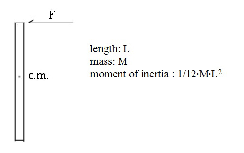
T = Ia'' where T is the applied torque, a'' is the acceleration of the angle of rotation of the object about its center of mass, and I the object's moment of inertial about its center of mass.
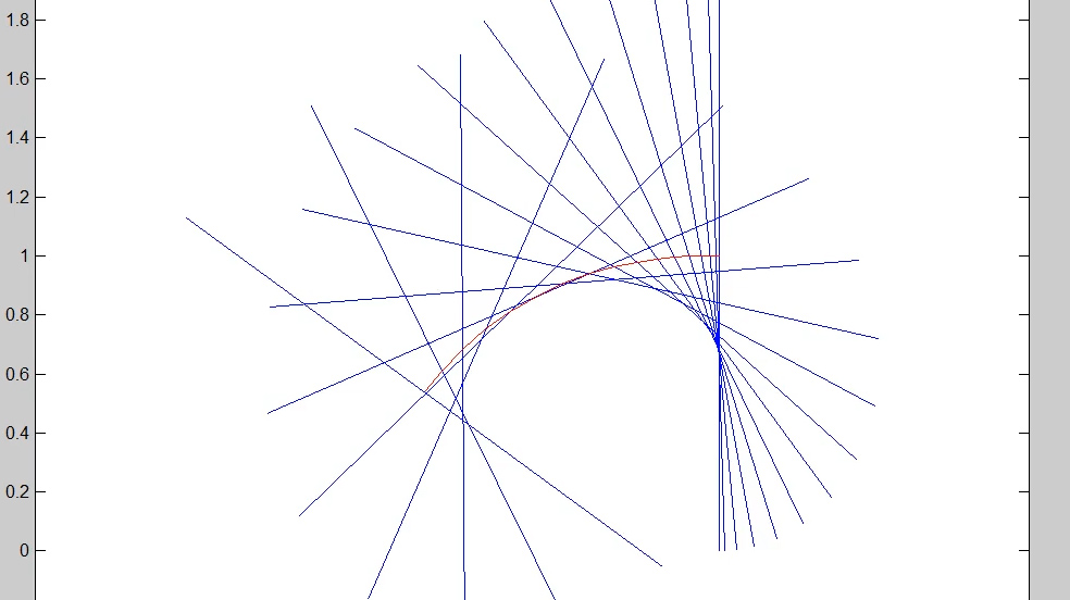
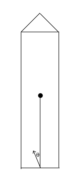
Applying a constant force perpendicular to the rod as shown will cause the center of mass to move in the direction of F as per F = MA and the rod will also rotate about its c.m. as per T = Ia''. The graph shows the motion of a tumbing rod, with the red line tracing its c.m. There was no gravity pulling the rod down.
We revisit the spring-box assembly, this time with an added hydraulic damper, similar to an automobile shock absorber. The photo shows a spring and damper combination. The force exerted by the damper is proportional to the velocity of the plunger in the damper and is C*p'(t) where c is the 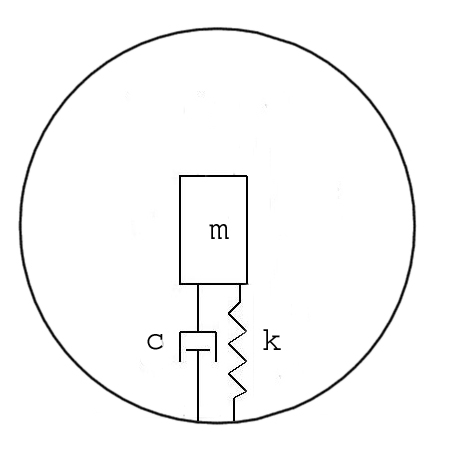 damping coefficient. The model of the spring-damper assembly is p''(t) = -k*p(t) - c*p'(t). Let's jump ahead a bit and put the spring-damper in a tennis ball that bounces and skids.
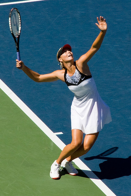
Then let's have Maria Sharapova give the ball a good whack, now the ball is traveling
through the air and spinning.
When the ball hits the ground it will skid and bounce; the skid is modeled as sliding friction, also called Couloumb friction, the model is simply F = -u*N*sign(v) where u is the coefficient of friction, N 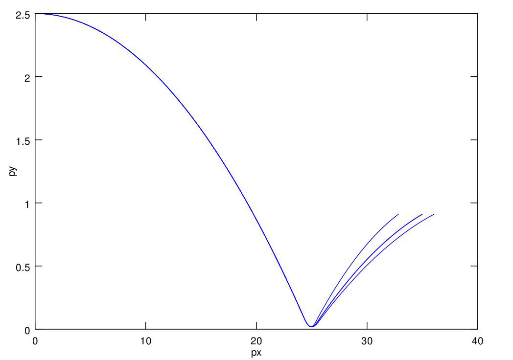 is the force (usually the weight) of the object on the surface, and sign(v) is 1 for v positive, 0 for v = 0, and -1 for v negative. Thus the magnitude of sliding friction is constant and it is in the direction opposite the apparent velocity of the ball on the surface. The skid generates a force which accelerates or decelerates the ball and which creates a torque which changes the spin rate.
Putting all the models together we can plot the trajectories for kick (topspin), flat, and slice (backspin) serves. This is all spelled out in detail in the book.
is the force (usually the weight) of the object on the surface, and sign(v) is 1 for v positive, 0 for v = 0, and -1 for v negative. Thus the magnitude of sliding friction is constant and it is in the direction opposite the apparent velocity of the ball on the surface. The skid generates a force which accelerates or decelerates the ball and which creates a torque which changes the spin rate.
Putting all the models together we can plot the trajectories for kick (topspin), flat, and slice (backspin) serves. This is all spelled out in detail in the book.
The spring-damper combination is used in motorcycle (shown) and auto suspension systems.

We have one axel (shown) and two axel models. For the one axel model the passenger just goes up and down. For the two axel model there is one spring-damper assembly of the back axel and one on the front,
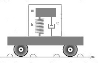 and the auto chassis is a rigid object acted on by gravity plus the forces of the two spring/shock absorbers, so it rocks.
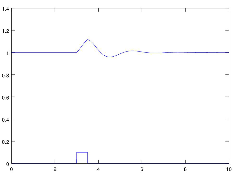
We can plot the up/down motion of the car when it hits a bump in the road. We program the bump just the way we programmed the impulse to the high-pass filter circuit above. The graph shows the bump in the road and the cars response to it. See the program here.
The forces acting on an airplane in flight are thrust, lift, drag, and gravity. In addition the pilot can activate control surfaces that generate force on the airplane. In order to study aircraft 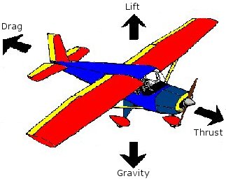 flight we need models these forces. Gravity we know, we will program thrust directly, and we will program one control torque, the torque resulting when an tail elevator is activated, directly. That leaves lift and drag.
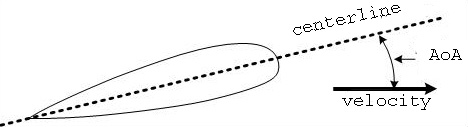
Lift and drag of an airplane depend on the airplane's angle of attack (AoA), that is the angle between the centerline of the airplane and the airplane's velocity vector, as shown.
The relationship between the lift coefficient (CL) and drag coefficient (CD) for a typical aircraft are shown in the figure. We model these functions with ad hoc piecewise linear functions and lift 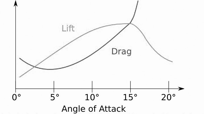 is determined using the formula, and a similar formula used for drag,
Lift = (1/2)*d*v2*s*CL where d=air density, v=velocity, s=wing surface area, CL = lift coefficient.
We initialize the mass, moment of inertia, and wing surface area from the data for a single-engine airplane, and we're ready to fly. Once we find the thrust that keeps us in level flight we have only 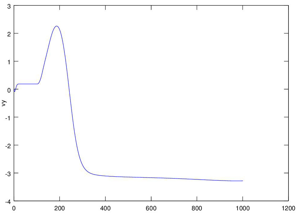 one control to activate, so we raise the tail elevator causing the tail to go down, the plane to go up, and then lose velocity and lift, and then go down as a result, as we see in the graph
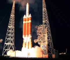
A rocket launched into orbit. In the previous projects we modeled the rocket as a point mass. Now we model it as a 2-D rigid body and we guide it by directing the thrust. The rocket is modeled on the Delta IV launch vehicle, a 2-stage rocket used for many satellite launches.
We guide the the first stage of the rocket by directing the thrust vector. As the rocket flies fuel is consumed, decreasing the rocket's mass and moment of inertia.
The rocket is launched from a location on the equator, and it inherits the earth horizontal velocity and angular rate. Unguided the rocket will fall back to earth. We guide the first stage so that the 2nd stage put the rocket into orbit.
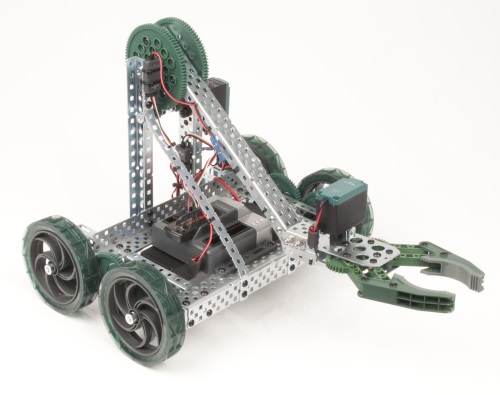
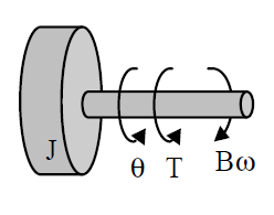
The VEX robot. A typical command for the VEX is to go 1 meter forward. The computer controlling the robot cannot issue that command to the robot directly as the computer only has control of the input voltage to the drive motor. We model both the circuit of the electric motor, and the dynamics of the robot to analyze the robot's performance.
The model for the motor circuit is shown, the motor generates torque T = Km·ia
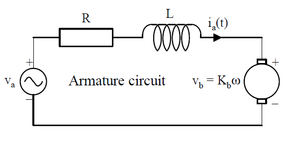
From Kirchoff's voltage law
va(t) = R·ia(t) + L·ia(t)’ + Ka·ω
so
ia(t)’=(va(t) - R·ia(t) - Kb· ω)/L
and the model for the robot axel is, from Newton's 2nd law for rotation, θ'' = ω’ = (T – B · ω )/ J = ( Km· ia – B · ω )/ (J + mK*r2) where J is the armature moment of inertia and B is the viscous damping coefficient of the rotor, mK is the mass of the kart and r is the radius of the kart wheel.
Adding an equation for θ to get axel position, the computational equations are
ia(t+dt) = ia(t+dt) + (va - R·ia - Kb· ω)/L*dt
ω(t+dt) = ω(t) + ( Km· ia - B· ω )/ (J + mK*r2) *dt
θ(t+dt) = θ(t) + ω(t)*dt
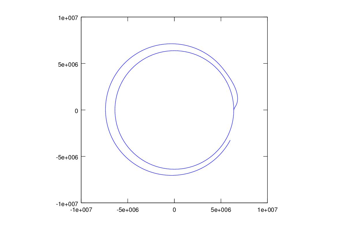
The robot can be run open loop, or the motor voltage can be controlled by a PID controller, i.e. a constant times the difference between the goal position and the current position. The graph shows the robot response with an underdamped P(not ID) controller (implemented as one assignement statement in the program).
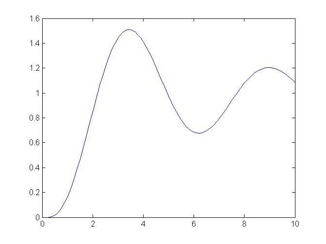
See the program here